This is a much bigger dataset than Crits-Christoph, with 6 billion reads spread out over 363 different samples. Interestingly, Nextflow seemed to struggle more with the number of samples than their size; when running the entire dataset through the pipeline I kept running into issues with caching that seemed to be due to the sheer number of jobs in the pipeline. I’ll keep working on these, but in the meantime I decided to separate the samples from the dataset into groups to make running them through the pipeline easier.
In this entry, I analyze the results of the pipeline on the 97 unenriched samples from the pipeline. These were collected from 9 California treatment plants between July 2020 and January 2021, pasteurized, filtered through a 0.22um filter and concentrated with 10-kDa Amicon filters. After this, they underwent RNA-seq library prep and were sequenced on an Illumina NovaSeq 6000.
The raw data
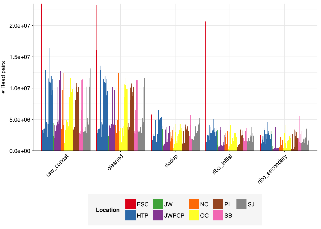
The Rothman unenriched samples totaled roughly 660M read pairs (151 gigabases of sequence). The number of reads per sample varied from 1.3M to 23.5M, with an average of 6.8M reads per sample. The number of reads per treatment plant varied from 6.7 to 165.9M, with an average of 73.3M.
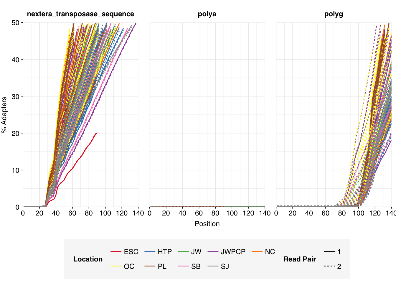
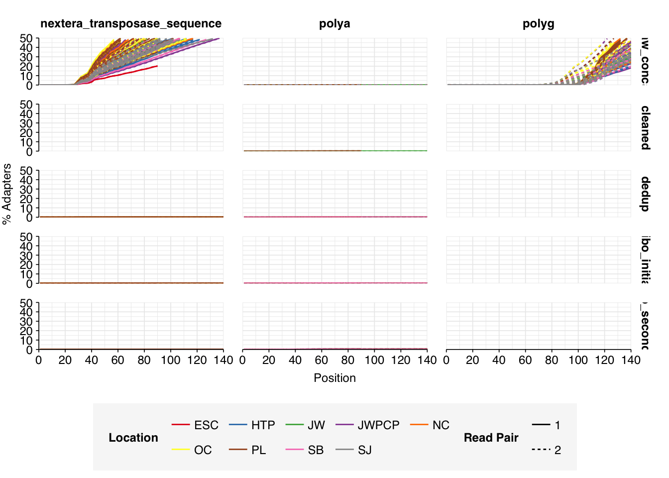
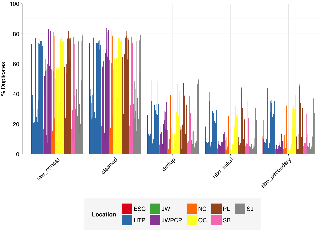
While many samples had low levels of sequence duplication according to FASTQC, others had very high levels of duplication in excess of 75%. The median level of duplication according to FASTQ was roughly 56%. Adapter levels were high.
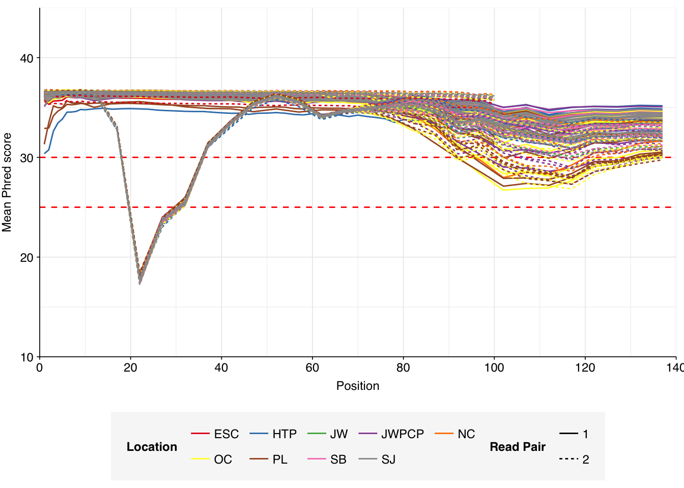
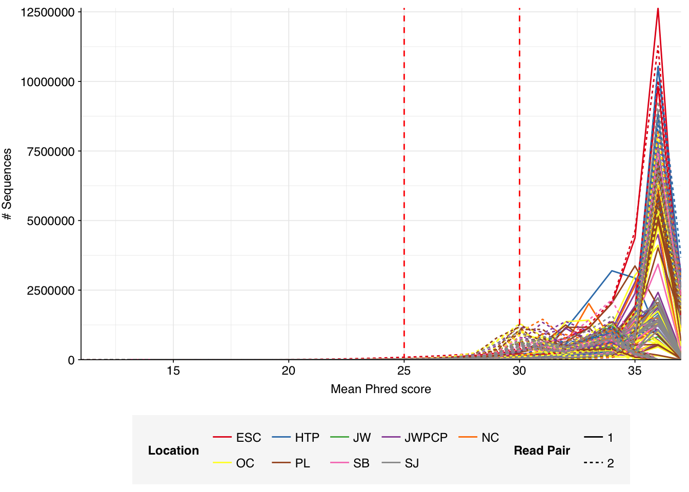
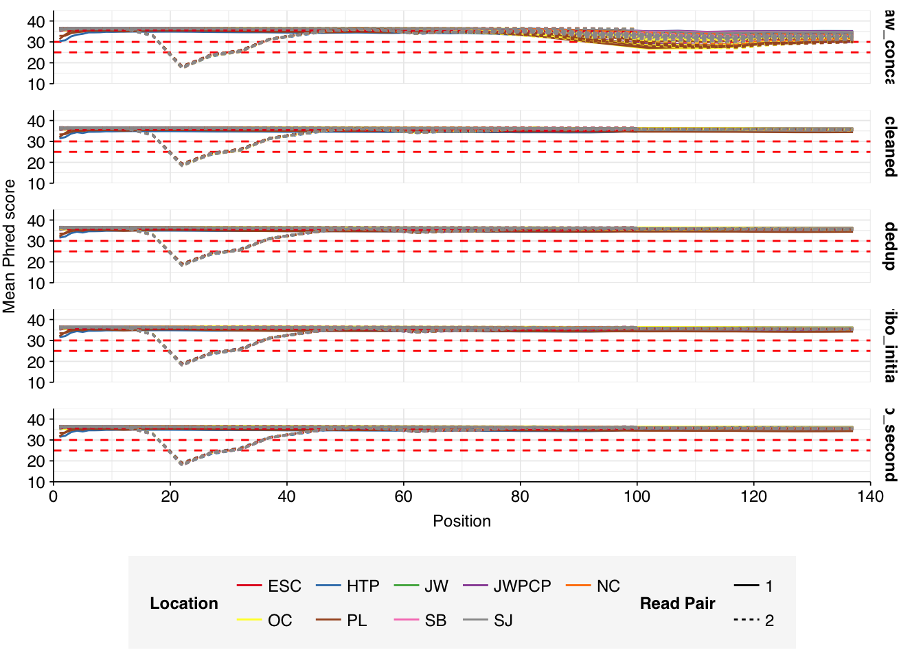
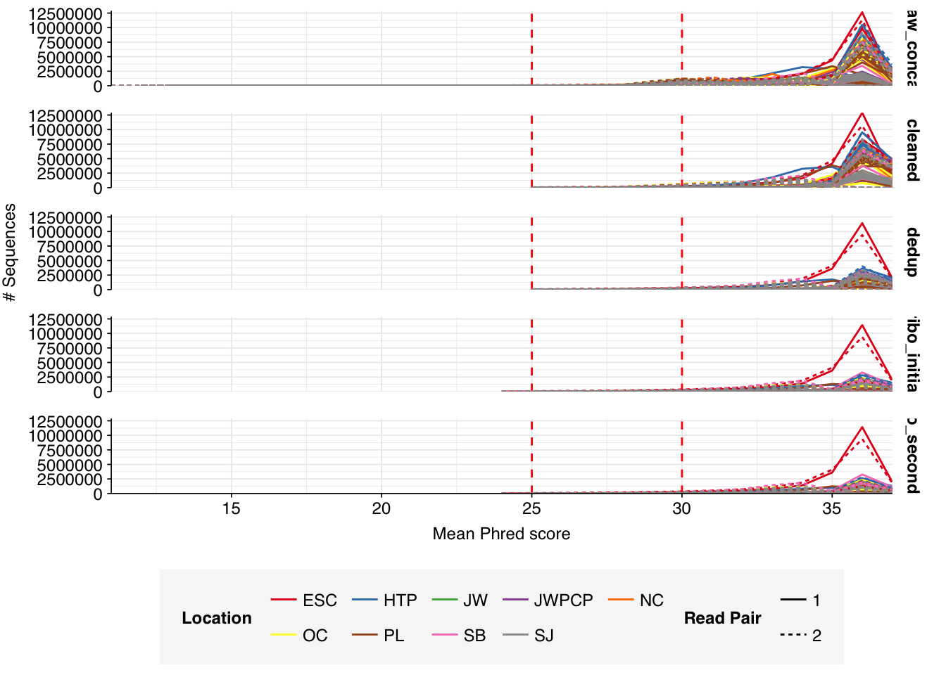
Read qualities for most samples were consistently very high, but some samples showed a large drop in sequence quality around position 20, suggesting a serious need for preprocessing to remove low-quality bases.
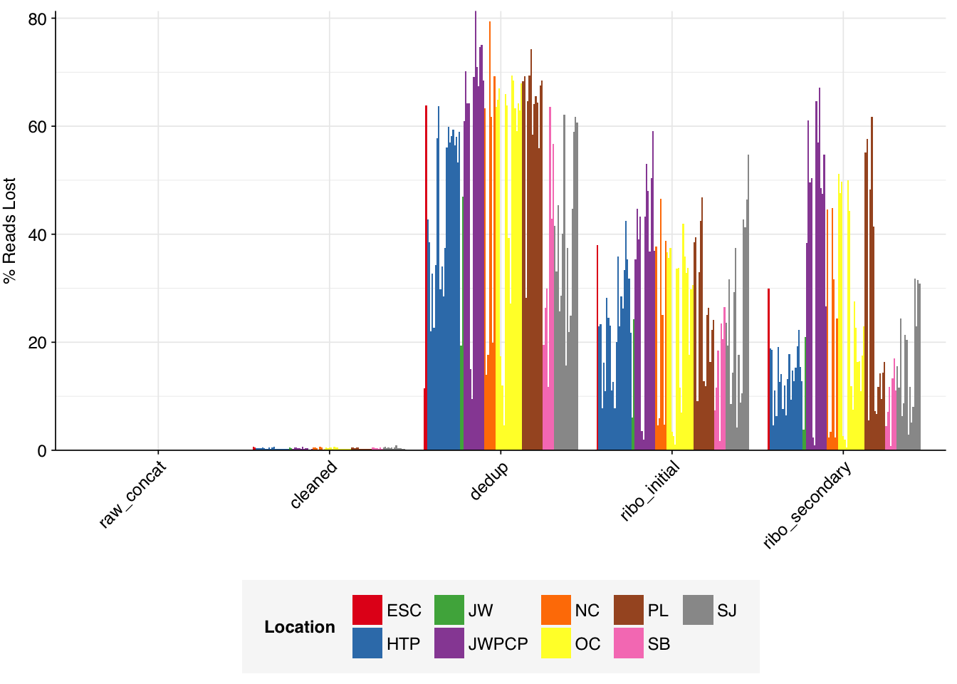
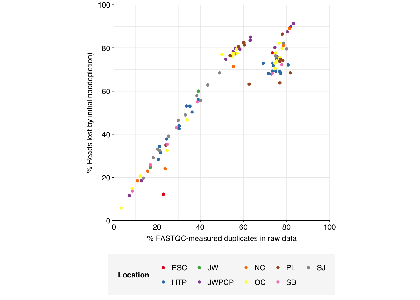
On average, cleaning, deduplication and conservative ribodepletion together removed about 60% of total reads from unenriched samples, with the largest reductions seen during deduplication. Secondary ribodepletion removing a further 6%. However, these summary figures conceal significant inter-sample variation. Unsurprisingly, samples that showed a higher initial level of duplication also showed greater read losses during preprocessing.
# Plot read losses vs initial duplication levelsg_loss_dup<-n_reads_rel%>%mutate(percent_duplicates_raw =percent_duplicates[1])%>%filter(stage=="ribo_initial")%>%ggplot(aes(x=percent_duplicates_raw, y=p_reads_lost_abs, color=location))+geom_point(shape =16)+scale_color_brewer(palette="Set1", name="Location")+scale_y_continuous("% Reads lost by initial ribodepletion)", expand=c(0,0), labels =function(x)x*100, breaks =seq(0,1,0.2), limits =c(0,1))+scale_x_continuous("% FASTQC-measured duplicates in raw data", expand=c(0,0), breaks =seq(0,100,20), limits=c(0,100))+theme_base+theme(aspect.ratio =1)g_loss_dup
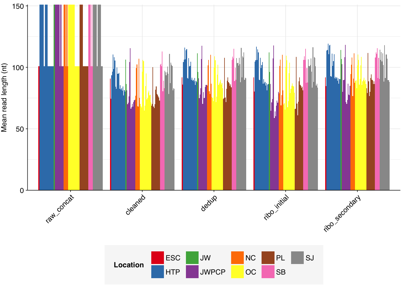
Data cleaning with FASTP was very successful at removing adapters, with no adapter sequences found by FASTQC at any stage after the raw data. Preprocessing successfully removed the terminal decline in quality seen in many samples, but failed to correct the large mid-read drop in quality seen in many samples. Since this group actually accounted for over half of samples, I decided to retain it for now, but will investigate ways to trim or discard such reads in future analyses, including of this data set.
Deduplication and ribodepletion were collectively quite effective at reducing measured duplicate levels, with the average detected duplication level after both processes reduced to roughly 14%. Note that the pipeline still doesn’t have a reverse-complement-sensitive deduplication pipeline, so only same-orientation duplicates have been removed.
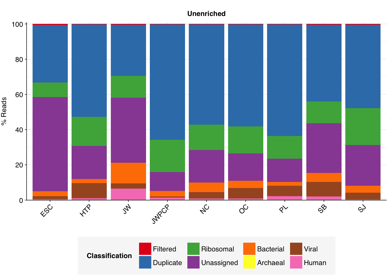
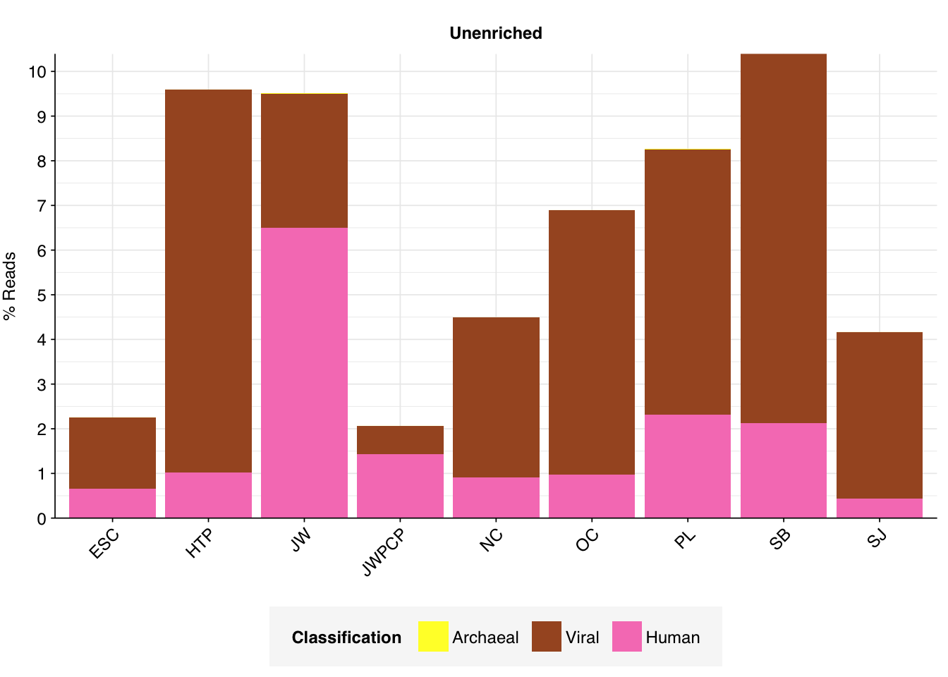
As before, to assess the high-level composition of the reads, I ran the ribodepleted files through Kraken (using the Standard 16 database) and summarized the results with Bracken. Combining these results with the read counts above gives us a breakdown of the inferred composition of the samples:
# Plot composition of minor componentsread_comp_minor<-read_comp_summ%>%filter(classification%in%c("Archaeal", "Viral", "Human", "Other"))palette_minor<-brewer.pal(9, "Set1")[6:9]g_comp_minor<-ggplot(read_comp_minor, aes(x=location, y=p_reads, fill=classification))+geom_col(position ="stack")+scale_y_continuous(name ="% Reads", breaks =seq(0,0.1,0.01), expand =c(0,0), labels =function(x)x*100)+scale_fill_manual(values=palette_minor, name ="Classification")+facet_wrap(.~enrichment, scales="free")+theme_kitg_comp_minor
Overall, in these unenriched samples, between 66% and 86% of reads (mean 74%) are low-quality, duplicates, or unassigned. Of the remainder, 8-21% (mean 15%) were identified as ribosomal, and 2-12% (mean 5%) were otherwise classified as bacterial. The fraction of human reads ranged from 0.4-6.5% (mean 1.8%) and that of viral reads from 0.6-8.6% (mean 4.5%).
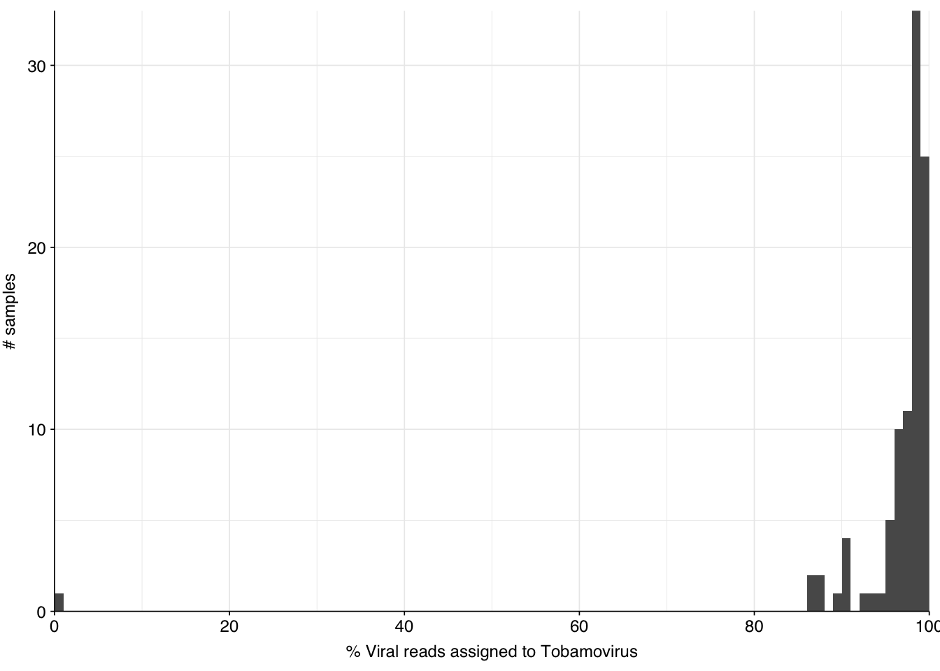
The latter of these is strikingly high, about an order of magnitude higher than that observed in Crits-Christoph. In the public dashboard, high levels of total virus reads are also observed, and attributed almost entirely to elevated levels of tobamoviruses, especially tomato brown rugose fruit virus. Digging into the Kraken reports for these samples, we find that for most samples, Tobamovirus indeed makes up the vast majority of viral reads:
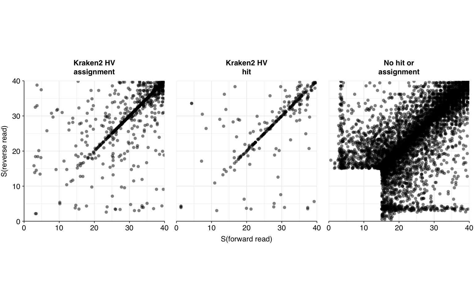
Next, I investigated the human-infecting virus read content of these unenriched samples, using a modified form of the pipeline used in my last entry:
After initial ribodepletion, surviving reads were aligned to a DB of human-infecting virus genomes with Bowtie2, using permissive alignment parameters.
Reads that aligned successfully with Bowtie2 were filtered to remove human, livestock, cloning vector, and other potential contaminant sequences, then run through Kraken2 using the standard 16GB database.
For surviving reads, the length-adjusted alignment score \(S=\frac{\text{bowtie2 alignment score}}{\ln(\text{read length})}\) was calculated, and reads were filtered out if they didn’t meet at least one of the following four criteria:
The read pair is assigned to a human-infecting virus by both Kraken and Bowtie2
The read pair contains a Kraken2 hit to the same taxid as it is assigned to by Bowtie2.
The read pair is unassigned by Kraken and \(S>15\) for the forward read
The read pair is unassigned by Kraken and \(S>15\) for the reverse read
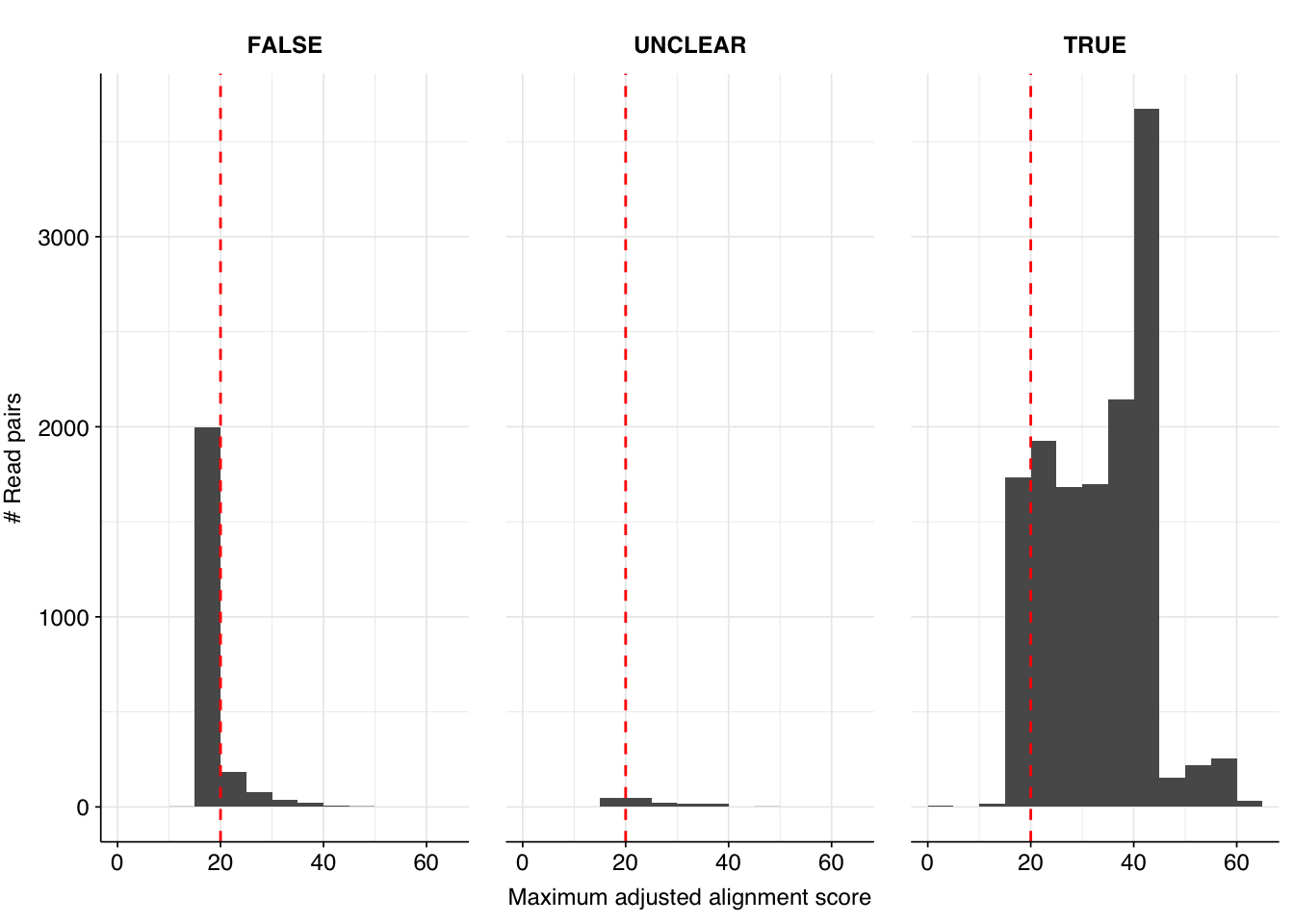
Applying all of these filtering steps leaves a total of 16034 read pairs across all unenriched samples (0.007% of surviving reads):
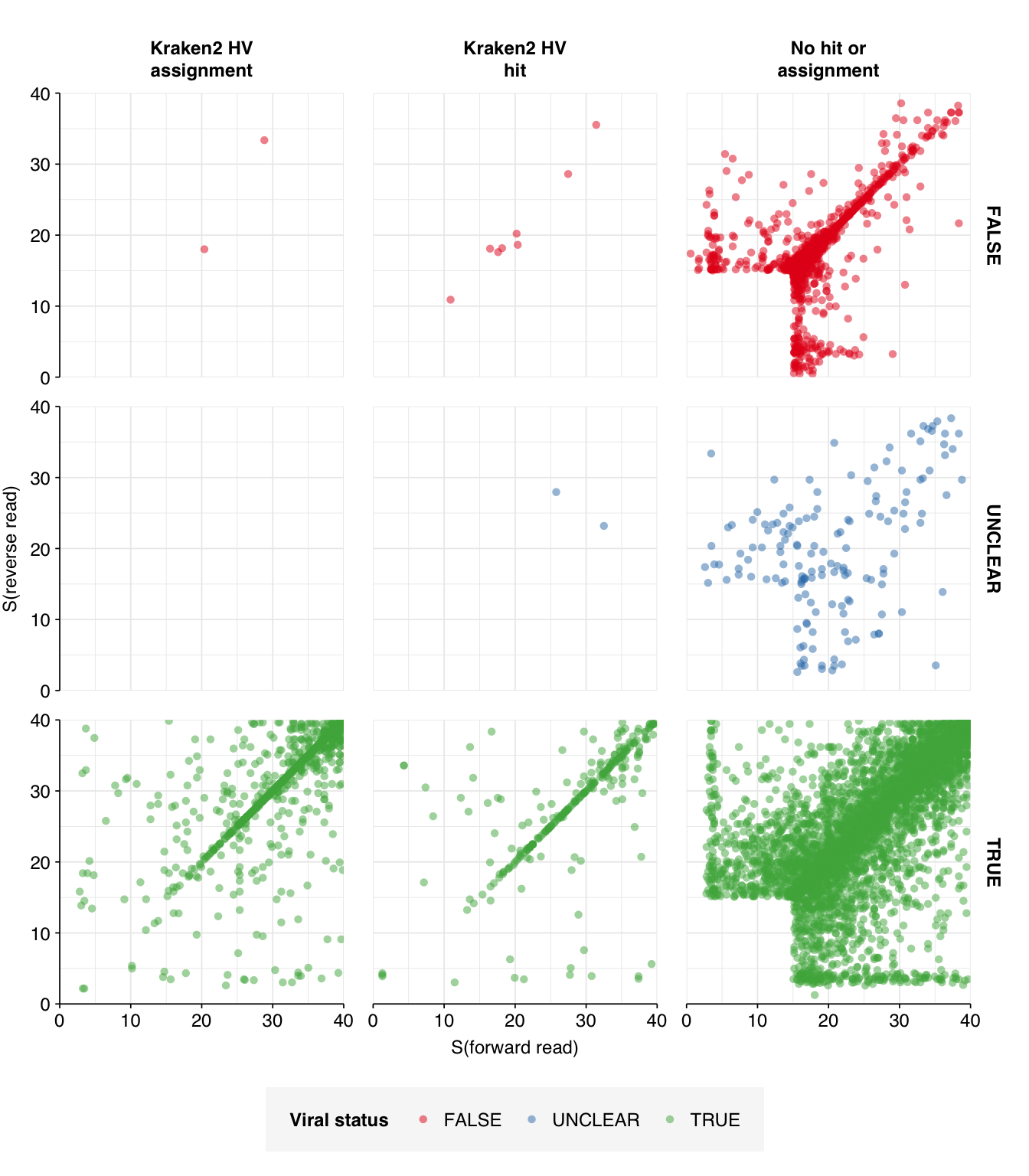
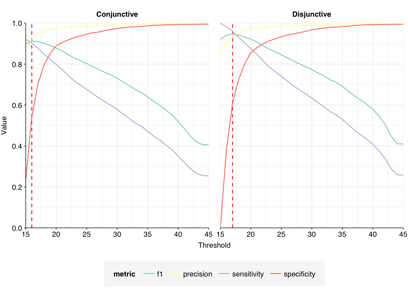
This initially looks pretty good, with high-scoring true-positives massively outnumbering false-positives and unclear cases. However, there are also a lot of low-scoring true-positives, which are excluded when the alignment score threshold is placed high enough to exclude the majority of false-positives. This pulls down sensitivity at higher score thresholds; as a result, F1 score is lower than I’d like, peaking at 0.947 for a disjunctive cutoff of 17 and dropping to 0.921 for a cutoff of 20.
Improving precision for high-scoring sequences will only have a marginal effect on F1 score here, as the limiting factor is sensitivity. The best way to improve this would be to find ways to better exclude low-scoring false-positives from the dataset, then lower the score threshold closer to 15. I’m wary about doing this, however, as I suspect low-scoring false-positives will be substantially harder to remove than high-scoring ones, and I’m somewhat less worried about false-negatives than false-positives here in any case. As such, I’m going to stick with my current pipeline for now.
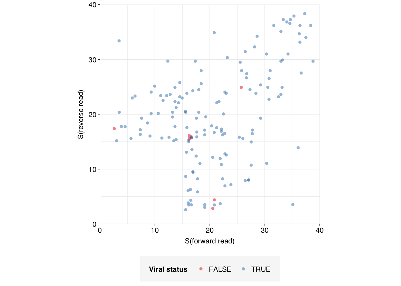
Moving on to the small number of “unclear” viral matches (155 total, 107 high-scoring), as with Crits-Christoph, the vast majority of these appear to be true positives when run on NCBI BLAST online:
Since this is two large datasets for which I’ve now gotten this result, I’ll henceforth treat reads for which only one of two reads shows a BLAST viral match as true positives for validation purposes.
Human-infecting virus reads: relative abundance
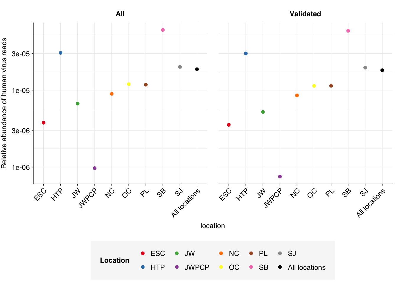
In total, my pipeline identified 12305 reads as human-viral out of 660M total reads, for a relative HV abundance of \(1.87 \times 10^{-5}\). This compares to \(4.3 \times 10^{-6}\) on the public dashboard, corresponding to the results for Kraken-only identification: a 4.4-fold increase, similar to that observed for Crits-Christoph. Excluding false-positives identified by BLAST above, the new estimate is reduced slightly, to \(1.81 \times 10^{-5}\).
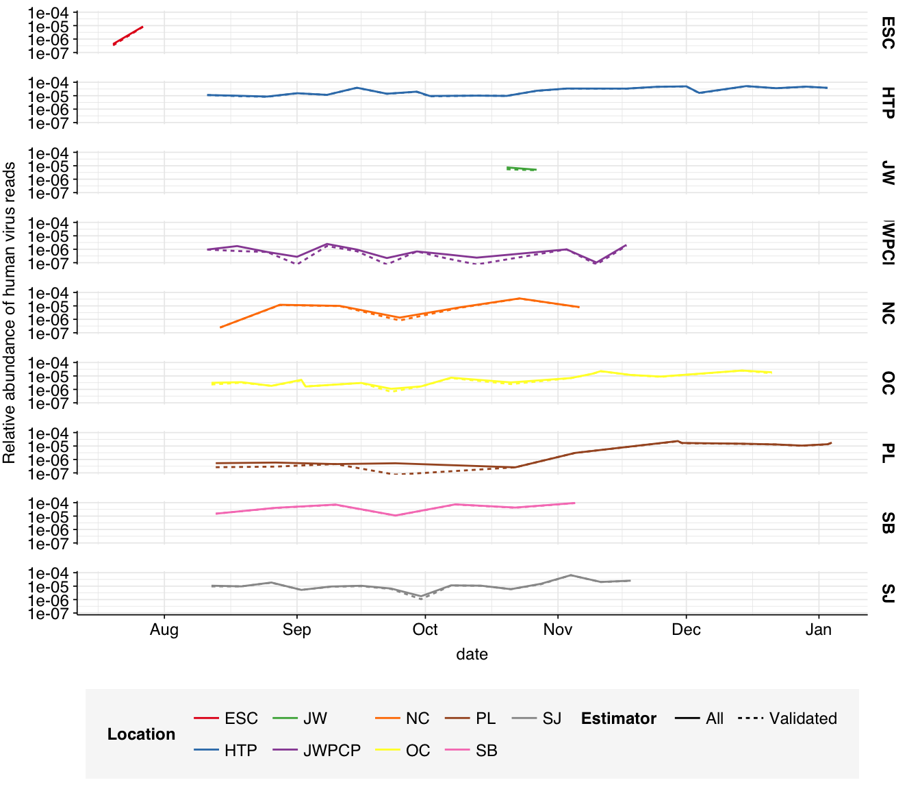
Aggregating by treatment plant location, we see substantial variation in HV relative abundance, from \(7.5 \times 10^{-7}\) for location JWPCP to \(5.91 \times 10^{-5}\) for location SB:
Plotting HV relative abundance over time for each plant, we see that while some plants remain roughly stable over time, several others exhibit a gradual increase in HV relative abundance over the course of the study, possibly related to the winter disease season:
Code
# Visualizeg_phv_time<-ggplot(read_counts_melted, aes(x=date, y=p, color=location, linetype=group))+geom_line()+scale_color_brewer(palette ="Set1", name="Location")+scale_y_log10("Relative abundance of human virus reads")+scale_linetype_discrete(name ="Estimator")+facet_grid(location~.)+theme_baseg_phv_time
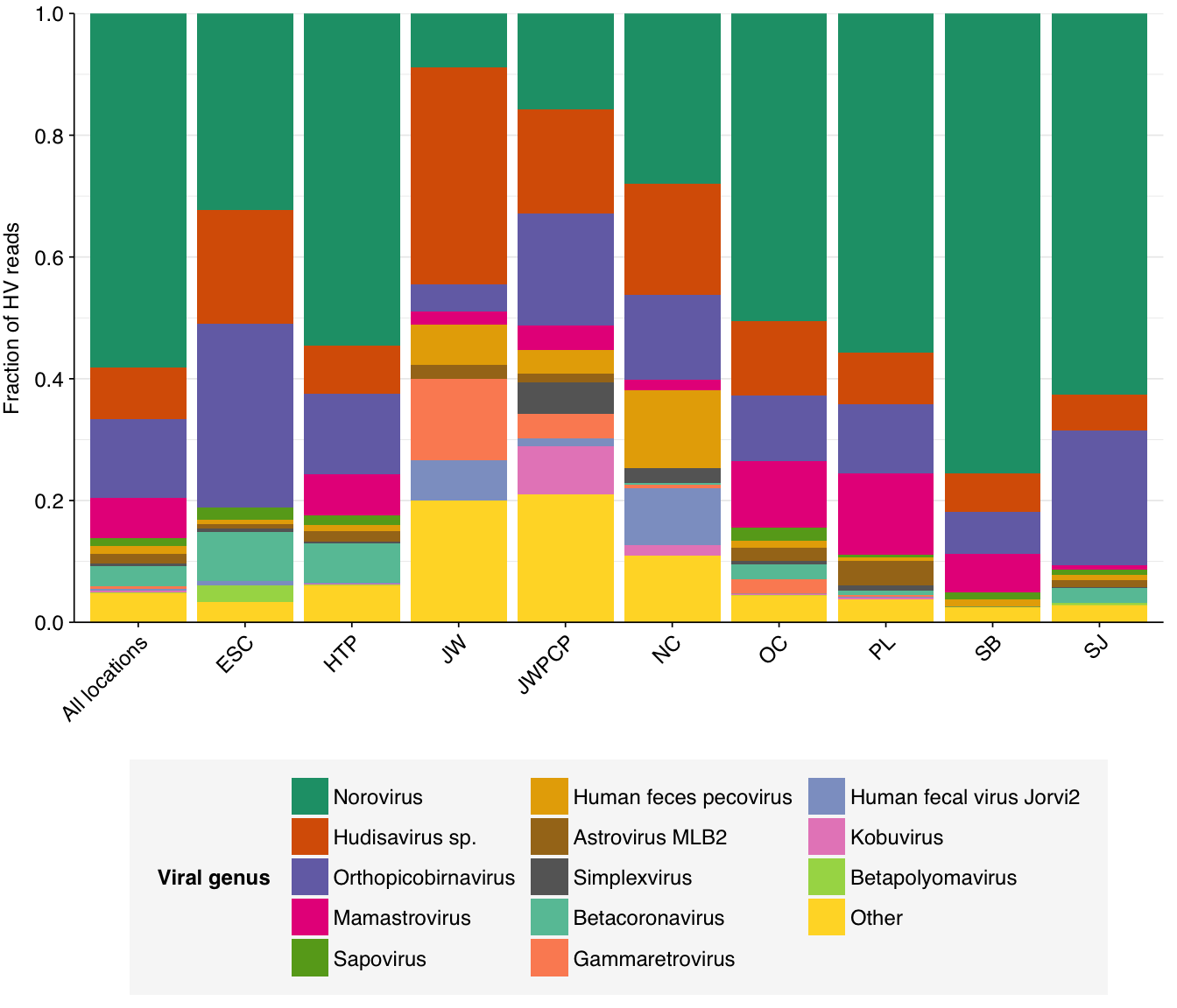
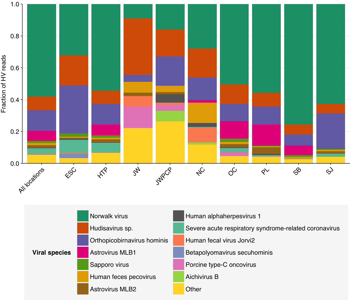
Digging into individual viruses, we see that fecal-oral viruses predominate, especially noroviruses (e.g. Norwalk virus) and hudisaviruses, though betacoronaviruses including SARS-CoV-2 make a respectable showing in several samples:
Code
# Get viral taxon names for putative HV readsmrg_hv_named<-mrg_hv%>%left_join(viral_taxa, by="taxid")# Discover viral species & genera for HV readsraise_rank<-function(read_db, taxid_db, out_rank="species", verbose=FALSE){# Get higher ranks than search rankranks<-c("subspecies", "species", "subgenus", "genus", "subfamily", "family", "suborder", "order", "class", "subphylum", "phylum", "kingdom", "superkingdom")rank_match<-which.max(ranks==out_rank)high_ranks<-ranks[rank_match:length(ranks)]# Merge read DB and taxid DBreads<-read_db%>%select(-parent_taxid, -rank, -name)%>%left_join(taxid_db, by="taxid")# Extract sequences that are already at appropriate rankreads_rank<-filter(reads, rank==out_rank)# Drop sequences at a higher rank and return unclassified sequencesreads_norank<-reads%>%filter(rank!=out_rank, !rank%in%high_ranks, !is.na(taxid))while(nrow(reads_norank)>0){# As long as there are unclassified sequences...# Promote read taxids and re-merge with taxid DB, then re-classify and filterreads_remaining<-reads_norank%>%mutate(taxid =parent_taxid)%>%select(-parent_taxid, -rank, -name)%>%left_join(taxid_db, by="taxid")reads_rank<-reads_remaining%>%filter(rank==out_rank)%>%bind_rows(reads_rank)reads_norank<-reads_remaining%>%filter(rank!=out_rank, !rank%in%high_ranks, !is.na(taxid))}# Finally, extract and append reads that were excluded during the processreads_dropped<-reads%>%filter(!seq_id%in%reads_rank$seq_id)reads_out<-reads_rank%>%bind_rows(reads_dropped)%>%select(-parent_taxid, -rank, -name)%>%left_join(taxid_db, by="taxid")return(reads_out)}hv_reads_species<-raise_rank(mrg_hv_named, viral_taxa, "species")hv_reads_genera<-raise_rank(mrg_hv_named, viral_taxa, "genus")# Count relative abundance for specieshv_species_counts_raw<-hv_reads_species%>%group_by(location, name)%>%summarize(n_reads_hv_all =sum(hv_status), n_reads_hv_validated =sum(hv_status&hv_true), .groups ="drop")%>%inner_join(read_counts_agg%>%select(location, n_reads_raw), by="location")hv_species_counts_all<-hv_species_counts_raw%>%group_by(name)%>%summarize(n_reads_hv_all =sum(n_reads_hv_all), n_reads_hv_validated =sum(n_reads_hv_validated), n_reads_raw =sum(n_reads_raw))%>%mutate(location ="All locations")hv_species_counts_agg<-bind_rows(hv_species_counts_raw, hv_species_counts_all)%>%mutate(p_reads_hv_all =n_reads_hv_all/n_reads_raw, p_reads_hv_validated =n_reads_hv_validated/n_reads_raw)# Count relative abundance for generahv_genera_counts_raw<-hv_reads_genera%>%group_by(location, name)%>%summarize(n_reads_hv_all =sum(hv_status), n_reads_hv_validated =sum(hv_status&hv_true), .groups ="drop")%>%inner_join(read_counts_agg%>%select(location, n_reads_raw), by="location")hv_genera_counts_all<-hv_genera_counts_raw%>%group_by(name)%>%summarize(n_reads_hv_all =sum(n_reads_hv_all), n_reads_hv_validated =sum(n_reads_hv_validated), n_reads_raw =sum(n_reads_raw))%>%mutate(location ="All locations")hv_genera_counts_agg<-bind_rows(hv_genera_counts_raw, hv_genera_counts_all)%>%mutate(p_reads_hv_all =n_reads_hv_all/n_reads_raw, p_reads_hv_validated =n_reads_hv_validated/n_reads_raw)
Code
# Compute ranks for species and genera and restrict to high-ranking taxamax_rank_species<-5max_rank_genera<-5hv_species_counts_ranked<-hv_species_counts_agg%>%group_by(location)%>%mutate(rank =rank(desc(n_reads_hv_all), ties.method="max"), highrank =rank<=max_rank_species)%>%group_by(name)%>%mutate(highrank_any =any(highrank), name_display =ifelse(highrank_any, name, "Other"))%>%group_by(name_display)%>%mutate(mean_rank =mean(rank))%>%arrange(mean_rank)%>%ungroup%>%mutate(name_display =fct_inorder(name_display))hv_genera_counts_ranked<-hv_genera_counts_agg%>%group_by(location)%>%mutate(rank =rank(desc(n_reads_hv_all), ties.method="max"), highrank =rank<=max_rank_genera)%>%group_by(name)%>%mutate(highrank_any =any(highrank), name_display =ifelse(highrank_any, name, "Other"))%>%group_by(name_display)%>%mutate(mean_rank =mean(rank))%>%arrange(mean_rank)%>%ungroup%>%mutate(name_display =fct_inorder(name_display))# Plot compositionpalette_rank<-c(brewer.pal(8, "Dark2"), brewer.pal(8, "Set2"))g_vcomp_genera<-ggplot(hv_genera_counts_ranked, aes(x=location, y=n_reads_hv_all, fill=name_display))+geom_col(position ="fill")+scale_fill_manual(values =palette_rank, name ="Viral genus")+scale_y_continuous(name ="Fraction of HV reads", breaks =seq(0,1,0.2), expand =c(0,0))+guides(fill =guide_legend(nrow=5))+theme_kitg_vcomp_species<-ggplot(hv_species_counts_ranked, aes(x=location, y=n_reads_hv_all, fill=name_display))+geom_col(position ="fill")+scale_fill_manual(values =palette_rank, name ="Viral species")+scale_y_continuous(name ="Fraction of HV reads", breaks =seq(0,1,0.2), expand =c(0,0))+guides(fill =guide_legend(nrow=7))+theme_kitg_vcomp_genera
Code
g_vcomp_species
These results make sense aren’t especially surprising. In my next entry, I’ll turn to the enriched samples from Rothman, and compare them to these unenriched samples.
Source Code
---title: "Workflow analysis of Rothman et al. (2021), part 1"subtitle: "Unenriched samples."author: "Will Bradshaw"date: 2024-02-27format: html: code-fold: true code-tools: true code-link: true df-print: pagededitor: visualtitle-block-banner: black---```{r}#| label: load-packages#| include: falselibrary(tidyverse)library(cowplot)library(patchwork)library(fastqcr)library(RColorBrewer)source("../scripts/aux_plot-theme.R")theme_base <- theme_base +theme(aspect.ratio =NULL)theme_kit <- theme_base +theme(axis.text.x =element_text(hjust =1, angle =45),axis.title.x =element_blank(),)tnl <-theme(legend.position ="none")```In my last entry, I finished workflow analysis of [Crits-Christoph et al. 2021](https://doi.org/10.1128%2FmBio.02703-20) enriched and unenriched MGS data. In this entry, I apply the workflow to another pre-existing dataset from the [P2RA project](https://naobservatory.org/reports/predicting-virus-relative-abundance-in-wastewater/), namely [Rothman et al. 2021](https://doi.org/10.1128/AEM.01448-21).This is a much bigger dataset than Crits-Christoph, with 6 billion reads spread out over 363 different samples. Interestingly, Nextflow seemed to struggle more with the number of samples than their size; when running the entire dataset through the pipeline I kept running into issues with caching that seemed to be due to the sheer number of jobs in the pipeline. I'll keep working on these, but in the meantime I decided to separate the samples from the dataset into groups to make running them through the pipeline easier.In this entry, I analyze the results of the pipeline on the 97 unenriched samples from the pipeline. These were collected from 9 California treatment plants between July 2020 and January 2021, pasteurized, filtered through a 0.22um filter and concentrated with 10-kDa Amicon filters. After this, they underwent RNA-seq library prep and were sequenced on an Illumina NovaSeq 6000.# The raw dataThe Rothman unenriched samples totaled roughly 660M read pairs (151 gigabases of sequence). The number of reads per sample varied from 1.3M to 23.5M, with an average of 6.8M reads per sample. The number of reads per treatment plant varied from 6.7 to 165.9M, with an average of 73.3M.While many samples had low levels of sequence duplication according to FASTQC, others had very high levels of duplication in excess of 75%. The median level of duplication according to FASTQ was roughly 56%. Adapter levels were high.Read qualities for most samples were consistently very high, but some samples showed a large drop in sequence quality around position 20, suggesting a serious need for preprocessing to remove low-quality bases.```{r}#| fig-height: 5#| warning: false# Data input pathsdata_dir <-"../data/2024-02-23_rothman-1/"libraries_path <-file.path(data_dir, "rothman-libraries-unenriched.csv")basic_stats_path <-file.path(data_dir, "qc_basic_stats.tsv")adapter_stats_path <-file.path(data_dir, "qc_adapter_stats.tsv")quality_base_stats_path <-file.path(data_dir, "qc_quality_base_stats.tsv")quality_seq_stats_path <-file.path(data_dir, "qc_quality_sequence_stats.tsv")# Import libraries and extract metadata from sample nameslibraries <-read_csv(libraries_path, show_col_types =FALSE) %>%separate(sample, c("location", "month", "day", "year", "x1", "x2"), remove =FALSE) %>%mutate(month =as.numeric(month), year =as.numeric(year), day =as.numeric(day),enrichment ="Unenriched", date =ymd(paste(year, month, day, sep="-"))) %>%select(-x1, -x2) %>%arrange(enrichment, location, date) %>%mutate(location =fct_inorder(location))# Import QC datastages <-c("raw_concat", "cleaned", "dedup", "ribo_initial", "ribo_secondary")basic_stats <-read_tsv(basic_stats_path, show_col_types =FALSE) %>%mutate(sample =sub("_2$", "", sample)) %>%inner_join(libraries, by="sample") %>%arrange(enrichment, location, date) %>%mutate(stage =factor(stage, levels = stages),sample =fct_inorder(sample))adapter_stats <-read_tsv(adapter_stats_path, show_col_types =FALSE) %>%mutate(sample =sub("_2$", "", sample)) %>%inner_join(libraries, by="sample") %>%mutate(stage =factor(stage, levels = stages),read_pair =fct_inorder(as.character(read_pair)))quality_base_stats <-read_tsv(quality_base_stats_path, show_col_types =FALSE) %>%mutate(sample =sub("_2$", "", sample)) %>%inner_join(libraries, by="sample") %>%mutate(stage =factor(stage, levels = stages),read_pair =fct_inorder(as.character(read_pair)))quality_seq_stats <-read_tsv(quality_seq_stats_path, show_col_types =FALSE) %>%mutate(sample =sub("_2$", "", sample)) %>%inner_join(libraries, by="sample") %>%mutate(stage =factor(stage, levels = stages),read_pair =fct_inorder(as.character(read_pair)))# Filter to raw databasic_stats_raw <- basic_stats %>%filter(stage =="raw_concat")adapter_stats_raw <- adapter_stats %>%filter(stage =="raw_concat")quality_base_stats_raw <- quality_base_stats %>%filter(stage =="raw_concat")quality_seq_stats_raw <- quality_seq_stats %>%filter(stage =="raw_concat")# Visualize basic statsg_nreads_raw <-ggplot(basic_stats_raw, aes(x=enrichment, y=n_read_pairs, fill=location, group=sample)) +geom_col(position="dodge") +scale_y_continuous(name="# Read pairs", expand=c(0,0)) +scale_fill_brewer(palette="Set1", name="Location") + theme_kitlegend_location <-get_legend(g_nreads_raw)g_nreads_raw_2 <- g_nreads_raw +theme(legend.position ="none")g_nbases_raw <-ggplot(basic_stats_raw, aes(x=enrichment, y=n_bases_approx, fill=location, group=sample)) +geom_col(position="dodge") +scale_y_continuous(name="Total base pairs (approx)", expand=c(0,0)) +scale_fill_brewer(palette="Set1", name="Location") + theme_kit +theme(legend.position ="none")g_ndup_raw <-ggplot(basic_stats_raw, aes(x=enrichment, y=percent_duplicates, fill=location, group=sample)) +geom_col(position="dodge") +scale_y_continuous(name="% Duplicates (FASTQC)", expand=c(0,0), limits =c(0,100), breaks =seq(0,100,20)) +scale_fill_brewer(palette="Set1", name="Location") + theme_kit +theme(legend.position ="none")g_basic_raw <-plot_grid(g_nreads_raw_2 + g_nbases_raw + g_ndup_raw, legend_location, ncol =1, rel_heights =c(1,0.1))g_basic_raw# Visualize adaptersg_adapters_raw <-ggplot(adapter_stats_raw, aes(x=position, y=pc_adapters, color=location, linetype = read_pair, group=interaction(sample, read_pair))) +geom_line() +scale_color_brewer(palette ="Set1", name ="Location") +scale_linetype_discrete(name ="Read Pair") +scale_y_continuous(name="% Adapters", limits=c(0,50),breaks =seq(0,50,10), expand=c(0,0)) +scale_x_continuous(name="Position", limits=c(0,140),breaks=seq(0,140,20), expand=c(0,0)) +guides(color=guide_legend(nrow=2,byrow=TRUE),linetype =guide_legend(nrow=2,byrow=TRUE)) +facet_wrap(~adapter) + theme_baseg_adapters_raw# Visualize qualityg_quality_base_raw <-ggplot(quality_base_stats_raw, aes(x=position, y=mean_phred_score, color=location, linetype = read_pair, group=interaction(sample,read_pair))) +geom_hline(yintercept=25, linetype="dashed", color="red") +geom_hline(yintercept=30, linetype="dashed", color="red") +geom_line() +scale_color_brewer(palette ="Set1", name ="Location") +scale_linetype_discrete(name ="Read Pair") +scale_y_continuous(name="Mean Phred score", expand=c(0,0), limits=c(10,45)) +scale_x_continuous(name="Position", limits=c(0,140),breaks=seq(0,140,20), expand=c(0,0)) +guides(color=guide_legend(nrow=2,byrow=TRUE),linetype =guide_legend(nrow=2,byrow=TRUE)) + theme_baseg_quality_seq_raw <-ggplot(quality_seq_stats_raw, aes(x=mean_phred_score, y=n_sequences, color=location, linetype = read_pair, group=interaction(sample,read_pair))) +geom_vline(xintercept=25, linetype="dashed", color="red") +geom_vline(xintercept=30, linetype="dashed", color="red") +geom_line() +scale_color_brewer(palette ="Set1", name ="Location") +scale_linetype_discrete(name ="Read Pair") +scale_x_continuous(name="Mean Phred score", expand=c(0,0)) +scale_y_continuous(name="# Sequences", expand=c(0,0)) +guides(color=guide_legend(nrow=2,byrow=TRUE),linetype =guide_legend(nrow=2,byrow=TRUE)) + theme_baseg_quality_base_rawg_quality_seq_raw```# PreprocessingOn average, cleaning, deduplication and conservative ribodepletion together removed about 60% of total reads from unenriched samples, with the largest reductions seen during deduplication. Secondary ribodepletion removing a further 6%. However, these summary figures conceal significant inter-sample variation. Unsurprisingly, samples that showed a higher initial level of duplication also showed greater read losses during preprocessing.```{r}#| warning: false# Plot reads over preprocessingg_reads_stages <-ggplot(basic_stats, aes(x=stage, y=n_read_pairs,fill=location,group=sample)) +geom_col(position="dodge") +scale_fill_brewer(palette="Set1", name="Location") +scale_y_continuous("# Read pairs", expand=c(0,0)) + theme_kitg_reads_stages# Plot relative read losses during preprocessingn_reads_rel <- basic_stats %>%select(sample, location, stage, enrichment, percent_duplicates, n_read_pairs) %>%group_by(sample, location, enrichment) %>%arrange(sample, location, enrichment, stage) %>%mutate(p_reads_retained = n_read_pairs /lag(n_read_pairs),p_reads_lost =1- p_reads_retained,p_reads_retained_abs = n_read_pairs / n_read_pairs[1],p_reads_lost_abs =1-p_reads_retained_abs)g_reads_rel <-ggplot(n_reads_rel, aes(x=stage, y=p_reads_lost,fill=location,group=sample)) +geom_col(position="dodge") +scale_fill_brewer(palette="Set1", name="Location") +scale_y_continuous("% Reads Lost", expand=c(0,0), labels =function(x) x*100) + theme_kitg_reads_rel# Plot read losses vs initial duplication levelsg_loss_dup <- n_reads_rel %>%mutate(percent_duplicates_raw = percent_duplicates[1]) %>%filter(stage =="ribo_initial") %>%ggplot(aes(x=percent_duplicates_raw, y=p_reads_lost_abs, color=location)) +geom_point(shape =16) +scale_color_brewer(palette="Set1", name="Location") +scale_y_continuous("% Reads lost by initial ribodepletion)", expand=c(0,0), labels =function(x) x*100, breaks =seq(0,1,0.2), limits =c(0,1)) +scale_x_continuous("% FASTQC-measured duplicates in raw data", expand=c(0,0),breaks =seq(0,100,20), limits=c(0,100)) + theme_base +theme(aspect.ratio =1)g_loss_dup```Data cleaning with FASTP was very successful at removing adapters, with no adapter sequences found by FASTQC at any stage after the raw data. Preprocessing successfully removed the terminal decline in quality seen in many samples, but failed to correct the large mid-read drop in quality seen in many samples. Since this group actually accounted for over half of samples, I decided to retain it for now, but will investigate ways to trim or discard such reads in future analyses, including of this data set.```{r}#| warning: false# Visualize adaptersg_adapters <-ggplot(adapter_stats, aes(x=position, y=pc_adapters, color=location, linetype = read_pair, group=interaction(sample, read_pair))) +geom_line() +scale_color_brewer(palette ="Set1", name ="Location") +scale_linetype_discrete(name ="Read Pair") +scale_y_continuous(name="% Adapters", limits=c(0,50),breaks =seq(0,50,10), expand=c(0,0)) +scale_x_continuous(name="Position", limits=c(0,140),breaks=seq(0,140,20), expand=c(0,0)) +guides(color=guide_legend(nrow=2,byrow=TRUE),linetype =guide_legend(nrow=2,byrow=TRUE)) +facet_grid(stage~adapter) + theme_baseg_adapters# Visualize qualityg_quality_base <-ggplot(quality_base_stats, aes(x=position, y=mean_phred_score, color=location, linetype = read_pair, group=interaction(sample,read_pair))) +geom_hline(yintercept=25, linetype="dashed", color="red") +geom_hline(yintercept=30, linetype="dashed", color="red") +geom_line() +scale_color_brewer(palette ="Set1", name ="Location") +scale_linetype_discrete(name ="Read Pair") +scale_y_continuous(name="Mean Phred score", expand=c(0,0), limits=c(10,45)) +scale_x_continuous(name="Position", limits=c(0,140),breaks=seq(0,140,20), expand=c(0,0)) +guides(color=guide_legend(nrow=2,byrow=TRUE),linetype =guide_legend(nrow=2,byrow=TRUE)) +facet_grid(stage~.) + theme_baseg_quality_seq <-ggplot(quality_seq_stats, aes(x=mean_phred_score, y=n_sequences, color=location, linetype = read_pair, group=interaction(sample,read_pair))) +geom_vline(xintercept=25, linetype="dashed", color="red") +geom_vline(xintercept=30, linetype="dashed", color="red") +geom_line() +scale_color_brewer(palette ="Set1", name ="Location") +scale_linetype_discrete(name ="Read Pair") +scale_x_continuous(name="Mean Phred score", expand=c(0,0)) +scale_y_continuous(name="# Sequences", expand=c(0,0)) +guides(color=guide_legend(nrow=2,byrow=TRUE),linetype =guide_legend(nrow=2,byrow=TRUE)) +facet_grid(stage~.) + theme_baseg_quality_baseg_quality_seq```Deduplication and ribodepletion were collectively quite effective at reducing measured duplicate levels, with the average detected duplication level after both processes reduced to roughly 14%. **Note that the pipeline still doesn't have a reverse-complement-sensitive deduplication pipeline, so only same-orientation duplicates have been removed.**```{r}g_dup_stages <-ggplot(basic_stats, aes(x=stage, y=percent_duplicates, fill=location, group=sample)) +geom_col(position="dodge") +scale_fill_brewer(palette ="Set1", name="Location") +scale_y_continuous("% Duplicates", limits=c(0,100), breaks=seq(0,100,20), expand=c(0,0)) + theme_kitg_readlen_stages <-ggplot(basic_stats, aes(x=stage, y=mean_seq_len, fill=location, group=sample)) +geom_col(position="dodge") +scale_fill_brewer(palette ="Set1", name="Location") +scale_y_continuous("Mean read length (nt)", expand=c(0,0)) + theme_kitlegend_loc <-get_legend(g_dup_stages)g_dup_stagesg_readlen_stages```# High-level compositionAs before, to assess the high-level composition of the reads, I ran the ribodepleted files through Kraken (using the Standard 16 database) and summarized the results with Bracken. Combining these results with the read counts above gives us a breakdown of the inferred composition of the samples:```{r}# Import Bracken databracken_path <-file.path(data_dir, "bracken_counts.tsv")bracken <-read_tsv(bracken_path, show_col_types =FALSE)total_assigned <- bracken %>%group_by(sample) %>%summarize(name ="Total",kraken_assigned_reads =sum(kraken_assigned_reads),added_reads =sum(added_reads),new_est_reads =sum(new_est_reads),fraction_total_reads =sum(fraction_total_reads))bracken_spread <- bracken %>%select(name, sample, new_est_reads) %>%mutate(name =tolower(name)) %>%pivot_wider(id_cols ="sample", names_from ="name", values_from ="new_est_reads")# Count readsread_counts_preproc <- basic_stats %>%select(sample, location, enrichment, stage, n_read_pairs) %>%pivot_wider(id_cols =c("sample", "location", "enrichment"), names_from="stage", values_from="n_read_pairs")read_counts <- read_counts_preproc %>%inner_join(total_assigned %>%select(sample, new_est_reads), by ="sample") %>%rename(assigned = new_est_reads) %>%inner_join(bracken_spread, by="sample")# Assess compositionread_comp <-transmute(read_counts, sample=sample, location=location,enrichment=enrichment,n_filtered = raw_concat-cleaned,n_duplicate = cleaned-dedup,n_ribosomal = (dedup-ribo_initial) + (ribo_initial-ribo_secondary),n_unassigned = ribo_secondary-assigned,n_bacterial = bacteria,n_archaeal = archaea,n_viral = viruses,n_human = eukaryota)read_comp_long <-pivot_longer(read_comp, -(sample:enrichment), names_to ="classification",names_prefix ="n_", values_to ="n_reads") %>%mutate(classification =fct_inorder(str_to_sentence(classification))) %>%group_by(sample) %>%mutate(p_reads = n_reads/sum(n_reads))read_comp_summ <- read_comp_long %>%group_by(location, enrichment, classification) %>%summarize(n_reads =sum(n_reads), .groups ="drop_last") %>%mutate(n_reads =replace_na(n_reads,0),p_reads = n_reads/sum(n_reads),pc_reads = p_reads*100)# Plot overall compositiong_comp <-ggplot(read_comp_summ, aes(x=location, y=p_reads, fill=classification)) +geom_col(position ="stack") +scale_y_continuous(name ="% Reads", limits =c(0,1.01), breaks =seq(0,1,0.2),expand =c(0,0), labels =function(x) x*100) +scale_fill_brewer(palette ="Set1", name ="Classification") +facet_wrap(.~enrichment, scales="free") + theme_kitg_comp# Plot composition of minor componentsread_comp_minor <- read_comp_summ %>%filter(classification %in%c("Archaeal", "Viral", "Human", "Other"))palette_minor <-brewer.pal(9, "Set1")[6:9]g_comp_minor <-ggplot(read_comp_minor, aes(x=location, y=p_reads, fill=classification)) +geom_col(position ="stack") +scale_y_continuous(name ="% Reads", breaks =seq(0,0.1,0.01),expand =c(0,0), labels =function(x) x*100) +scale_fill_manual(values=palette_minor, name ="Classification") +facet_wrap(.~enrichment, scales="free") + theme_kitg_comp_minor```Overall, in these unenriched samples, between 66% and 86% of reads (mean 74%) are low-quality, duplicates, or unassigned. Of the remainder, 8-21% (mean 15%) were identified as ribosomal, and 2-12% (mean 5%) were otherwise classified as bacterial. The fraction of human reads ranged from 0.4-6.5% (mean 1.8%) and that of viral reads from 0.6-8.6% (mean 4.5%).The latter of these is strikingly high, about an order of magnitude higher than that observed in Crits-Christoph. In the [public dashboard](https://data.securebio.org/mgs-counts/), high levels of total virus reads are also observed, and attributed almost entirely to elevated levels of tobamoviruses, especially tomato brown rugose fruit virus. Digging into the Kraken reports for these samples, we find that for most samples, *Tobamovirus* indeed makes up the vast majority of viral reads:```{r}toba_path <-file.path(data_dir, "tobamovirus.tsv")toba <-read_tsv(toba_path, show_col_types =FALSE)g_toba <-ggplot(toba, aes(x=p_viral_reads_Tobamovirus)) +geom_histogram(binwidth =0.01, boundary=0) +scale_x_continuous(name ="% Viral reads assigned to Tobamovirus",limits =c(0,1), breaks =seq(0,1,0.2), expand =c(0,0),labels =function(x) x*100) +scale_y_continuous("# samples", breaks =seq(0,100,10),expand =c(0,0)) + theme_baseg_toba```# Human-infecting virus reads: validationNext, I investigated the human-infecting virus read content of these unenriched samples, using a modified form of the pipeline used in my last entry:1. After initial ribodepletion, surviving reads were aligned to a DB of human-infecting virus genomes with Bowtie2, using permissive alignment parameters.2. Reads that aligned successfully with Bowtie2 were filtered to remove human, livestock, cloning vector, and other potential contaminant sequences, then run through Kraken2 using the standard 16GB database.3. For surviving reads, the length-adjusted alignment score $S=\frac{\text{bowtie2 alignment score}}{\ln(\text{read length})}$ was calculated, and reads were filtered out if they didn't meet at least one of the following four criteria: - The read pair is *assigned* to a human-infecting virus by both Kraken and Bowtie2 - The read pair contains a Kraken2 *hit* to the same taxid as it is assigned to by Bowtie2. - The read pair is unassigned by Kraken and $S>15$ for the forward read - The read pair is unassigned by Kraken and $S>15$ for the reverse readApplying all of these filtering steps leaves a total of 16034 read pairs across all unenriched samples (0.007% of surviving reads):```{r}hv_reads_filtered_path <-file.path(data_dir, "hv_hits_putative_filtered.tsv.gz")hv_reads_filtered <-read_tsv(hv_reads_filtered_path, show_col_types =FALSE) %>%inner_join(libraries, by="sample") %>%arrange(enrichment, location, date) %>%mutate(sample =fct_inorder(sample))n_hv_filtered <- hv_reads_filtered %>%group_by(sample, location, enrichment) %>% count %>%inner_join(basic_stats %>%filter(stage =="ribo_initial") %>%select(sample, n_read_pairs), by="sample") %>%rename(n_putative = n, n_total = n_read_pairs) %>%mutate(p_reads = n_putative/n_total, pc_reads = p_reads *100)``````{r}#| warning: false#| fig-width: 8mrg <- hv_reads_filtered %>%mutate(kraken_label =ifelse(assigned_hv, "Kraken2 HV\nassignment",ifelse(hit_hv, "Kraken2 HV\nhit","No hit or\nassignment"))) %>%group_by(sample) %>%arrange(desc(adj_score_fwd), desc(adj_score_rev)) %>%mutate(seq_num =row_number(),adj_score_max =pmax(adj_score_fwd, adj_score_rev))# Import Bowtie2/Kraken data and perform filtering stepsg_mrg <-ggplot(mrg, aes(x=adj_score_fwd, y=adj_score_rev)) +geom_point(alpha=0.5, shape=16) +scale_x_continuous(name="S(forward read)", limits=c(0,40), breaks=seq(0,100,10), expand =c(0,0)) +scale_y_continuous(name="S(reverse read)", limits=c(0,40), breaks=seq(0,100,10), expand =c(0,0)) +facet_wrap(~kraken_label, labeller =labeller(kit =label_wrap_gen(20))) + theme_base +theme(aspect.ratio=1)g_mrg```To investigate these putative viral reads, I ran them through BLASTN and analyzed the results in a similar manner to Crits-Christoph:```{r}mrg_num <- mrg %>%group_by(sample) %>%arrange(sample, desc(adj_score_max)) %>%mutate(seq_num =row_number(), seq_head =paste0(">", sample, "_", seq_num))mrg_fasta <- mrg_num %>% ungroup %>%select(header1=seq_head, seq1=query_seq_fwd, header2=seq_head, seq2=query_seq_rev) %>%mutate(header1=paste0(header1, "_1"), header2=paste0(header2, "_2"))mrg_fasta_out <-do.call(paste, c(mrg_fasta, sep="\n")) %>%paste(collapse="\n")write(mrg_fasta_out, file.path(data_dir, "rothman-putative-viral.fasta"))``````{r}#| warning: false# Import viral taxids and relationshipsviral_taxa_path <-file.path(data_dir, "viral-taxa.tsv.gz")viral_taxa <-read_tsv(viral_taxa_path, show_col_types =FALSE)# Import BLAST resultsblast_results_path <-file.path(data_dir, "rothman-putative-viral.blast.gz")blast_cols <-c("qseqid", "sseqid", "sgi", "staxid", "qlen", "evalue", "bitscore", "qcovs", "length", "pident", "mismatch", "gapopen", "sstrand", "qstart", "qend", "sstart", "send")blast_results <-read_tsv(blast_results_path, show_col_types =FALSE, col_names = blast_cols, col_types =cols(.default="c"))# Add viral statusblast_results_viral <-mutate(blast_results, viral = staxid %in% viral_taxa$taxid)# Filter for best hit for each query/subject, then rank hits for each queryblast_results_best <- blast_results_viral %>%group_by(qseqid, staxid) %>%filter(bitscore ==max(bitscore)) %>%filter(length ==max(length)) %>%filter(row_number() ==1)blast_results_ranked <- blast_results_best %>%group_by(qseqid) %>%mutate(rank =dense_rank(desc(bitscore)))blast_results_highrank <- blast_results_ranked %>%filter(rank <=5) %>%mutate(read_pair =str_split(qseqid, "_") %>%sapply(nth, n=-1), seq_num =str_split(qseqid, "_") %>%sapply(nth, n=-2), sample =str_split(qseqid, "_") %>%lapply(head, n=-2) %>%sapply(paste, collapse="_")) %>%mutate(bitscore =as.numeric(bitscore), seq_num =as.numeric(seq_num))# Summarize by read pair and taxidblast_results_paired <- blast_results_highrank %>%group_by(sample, seq_num, staxid, viral) %>%summarize(bitscore_max =max(bitscore), bitscore_min =min(bitscore),n_reads =n(), .groups ="drop") %>%mutate(viral_full = viral & n_reads ==2)# Compare to Kraken & Bowtie assignmentsmrg_assign <- mrg_num %>%select(sample, seq_num, taxid, assigned_taxid)blast_results_assign <-left_join(blast_results_paired, mrg_assign, by=c("sample", "seq_num")) %>%mutate(taxid_match_bowtie = (staxid == taxid),taxid_match_kraken = (staxid == assigned_taxid),taxid_match_any = taxid_match_bowtie | taxid_match_kraken)blast_results_out <- blast_results_assign %>%group_by(sample, seq_num) %>%summarize(viral_status =ifelse(any(viral_full), 2,ifelse(any(taxid_match_any), 2,ifelse(any(viral), 1, 0))),.groups ="drop")``````{r}#| fig-height: 8#| warning: false# Merge BLAST results with unenriched read datamrg_blast <-full_join(mrg_num, blast_results_out, by=c("sample", "seq_num")) %>%mutate(viral_status =replace_na(viral_status, 0),viral_status_out =ifelse(viral_status ==0, "FALSE",ifelse(viral_status ==1, "UNCLEAR", "TRUE")),viral_status_out =factor(viral_status_out, levels =c("FALSE", "UNCLEAR", "TRUE")))# Plotg_mrg_blast_0 <- mrg_blast %>%ggplot(aes(x=adj_score_fwd, y=adj_score_rev, color=viral_status_out)) +geom_point(alpha=0.5, shape=16) +scale_x_continuous(name="S(forward read)", limits=c(0,40), breaks=seq(0,100,10), expand =c(0,0)) +scale_y_continuous(name="S(reverse read)", limits=c(0,40), breaks=seq(0,100,10), expand =c(0,0)) +scale_color_brewer(palette ="Set1", name ="Viral status") +facet_grid(viral_status_out~kraken_label, labeller =labeller(kit =label_wrap_gen(20))) + theme_base +theme(aspect.ratio=1)g_mrg_blast_0``````{r}g_hist_0 <-ggplot(mrg_blast, aes(x=adj_score_max)) +geom_histogram(binwidth=5,boundary=0,position="dodge") +facet_wrap(~viral_status_out) +scale_x_continuous(name ="Maximum adjusted alignment score") +scale_y_continuous(name="# Read pairs") +scale_fill_brewer(palette ="Dark2") + theme_base +geom_vline(xintercept=20, linetype="dashed", color="red")g_hist_0```This initially looks pretty good, with high-scoring true-positives massively outnumbering false-positives and unclear cases. However, there are also a lot of *low*-scoring true-positives, which are excluded when the alignment score threshold is placed high enough to exclude the majority of false-positives. This pulls down sensitivity at higher score thresholds; as a result, F1 score is lower than I'd like, peaking at 0.947 for a disjunctive cutoff of 17 and dropping to 0.921 for a cutoff of 20.```{r}test_sens_spec <-function(tab, score_threshold, conjunctive, include_special){if (!include_special) tab <-filter(tab, viral_status_out %in%c("TRUE", "FALSE")) tab_retained <- tab %>%mutate(conjunctive = conjunctive,retain_score_conjunctive = (adj_score_fwd > score_threshold & adj_score_rev > score_threshold), retain_score_disjunctive = (adj_score_fwd > score_threshold | adj_score_rev > score_threshold),retain_score =ifelse(conjunctive, retain_score_conjunctive, retain_score_disjunctive),retain = assigned_hv | hit_hv | retain_score) %>%group_by(viral_status_out, retain) %>% count pos_tru <- tab_retained %>%filter(viral_status_out =="TRUE", retain) %>%pull(n) %>% sum pos_fls <- tab_retained %>%filter(viral_status_out !="TRUE", retain) %>%pull(n) %>% sum neg_tru <- tab_retained %>%filter(viral_status_out !="TRUE", !retain) %>%pull(n) %>% sum neg_fls <- tab_retained %>%filter(viral_status_out =="TRUE", !retain) %>%pull(n) %>% sum sensitivity <- pos_tru / (pos_tru + neg_fls) specificity <- neg_tru / (neg_tru + pos_fls) precision <- pos_tru / (pos_tru + pos_fls) f1 <-2* precision * sensitivity / (precision + sensitivity) out <-tibble(threshold=score_threshold, include_special = include_special, conjunctive = conjunctive, sensitivity=sensitivity, specificity=specificity, precision=precision, f1=f1)return(out)}range_f1 <-function(intab, inc_special, inrange=15:45){ tss <- purrr::partial(test_sens_spec, tab=intab, include_special=inc_special) stats_conj <-lapply(inrange, tss, conjunctive=TRUE) %>% bind_rows stats_disj <-lapply(inrange, tss, conjunctive=FALSE) %>% bind_rows stats_all <-bind_rows(stats_conj, stats_disj) %>%pivot_longer(!(threshold:conjunctive), names_to="metric", values_to="value") %>%mutate(conj_label =ifelse(conjunctive, "Conjunctive", "Disjunctive"))return(stats_all)}inc_special <-FALSEstats_0 <-range_f1(mrg_blast, inc_special) %>%mutate(attempt=0)threshold_opt_0 <- stats_0 %>%group_by(conj_label,attempt) %>%filter(metric =="f1") %>%filter(value ==max(value)) %>%filter(threshold ==min(threshold))g_stats_0 <-ggplot(stats_0, aes(x=threshold, y=value, color=metric)) +geom_vline(data = threshold_opt_0, mapping =aes(xintercept=threshold),color ="red", linetype ="dashed") +geom_line() +scale_y_continuous(name ="Value", limits=c(0,1), breaks =seq(0,1,0.2), expand =c(0,0)) +scale_x_continuous(name ="Threshold", expand =c(0,0)) +scale_color_brewer(palette="Set3") +facet_wrap(~conj_label) + theme_baseg_stats_0```Improving precision for high-scoring sequences will only have a marginal effect on F1 score here, as the limiting factor is sensitivity. The best way to improve this would be to find ways to better exclude low-scoring false-positives from the dataset, then lower the score threshold closer to 15. I'm wary about doing this, however, as I suspect low-scoring false-positives will be substantially harder to remove than high-scoring ones, and I'm somewhat less worried about false-negatives than false-positives here in any case. As such, I'm going to stick with my current pipeline for now.```{r}mrg_unclear <- mrg_blast %>% ungroup %>%filter(viral_status_out =="UNCLEAR") %>%arrange(sample, seq_num)mrg_unclear_fasta <- mrg_unclear %>%select(header1=seq_head, seq1=query_seq_fwd, header2=seq_head, seq2=query_seq_rev) %>%mutate(header1=paste0(header1, "_1"), header2=paste0(header2, "_2"))mrg_unclear_fasta_out <-do.call(paste, c(mrg_unclear_fasta, sep="\n")) %>%paste(collapse="\n")write(mrg_unclear_fasta_out, file.path(data_dir, "rothman-unclear-viral.fasta"))```Moving on to the small number of "unclear" viral matches (155 total, 107 high-scoring), as with Crits-Christoph, the vast majority of these appear to be true positives when run on NCBI BLAST online:```{r}#| warning: falseunclear_viral_status <-c(rep(TRUE, 53), FALSE, TRUE,rep(TRUE, 13), FALSE, rep(TRUE, 15), FALSE, rep(TRUE, 6), FALSE, rep(TRUE, 12), FALSE, rep(TRUE, 5),rep(TRUE, 2), FALSE, rep(TRUE, 12), FALSE, rep(TRUE, 29))mrg_unclear_out <- mrg_unclear %>%mutate(viral_status_true = unclear_viral_status)g_unclear <- mrg_unclear_out %>%ggplot(aes(x=adj_score_fwd, y=adj_score_rev, color=viral_status_true)) +geom_point(alpha=0.5, shape=16) +scale_x_continuous(name="S(forward read)", limits=c(0,40), breaks=seq(0,100,10), expand =c(0,0)) +scale_y_continuous(name="S(reverse read)", limits=c(0,40), breaks=seq(0,100,10), expand =c(0,0)) +scale_color_brewer(palette ="Set1", name ="Viral status") + theme_base +theme(aspect.ratio=1)g_unclear```Since this is two large datasets for which I've now gotten this result, I'll henceforth treat reads for which only one of two reads shows a BLAST viral match as true positives for validation purposes.# Human-infecting virus reads: relative abundanceIn total, my pipeline identified 12305 reads as human-viral out of 660M total reads, for a relative HV abundance of $1.87 \times 10^{-5}$. This compares to $4.3 \times 10^{-6}$ on the public dashboard, corresponding to the results for Kraken-only identification: a 4.4-fold increase, similar to that observed for Crits-Christoph. Excluding false-positives identified by BLAST above, the new estimate is reduced slightly, to $1.81 \times 10^{-5}$.Aggregating by treatment plant location, we see substantial variation in HV relative abundance, from $7.5 \times 10^{-7}$ for location JWPCP to $5.91 \times 10^{-5}$ for location SB:```{r}# Get raw read countsread_counts_raw <- basic_stats %>%filter(stage =="raw_concat") %>%select(sample, location, date, n_reads_raw = n_read_pairs)# Get HV read counts & RAmrg_hv <- mrg_blast %>%mutate(hv_status = assigned_hv | hit_hv | adj_score_max >=20,hv_true = viral_status >=1)read_counts_hv_all <- mrg_hv %>%filter(hv_status) %>%group_by(sample) %>%count(name ="n_reads_hv_all")read_counts_hv_val <- mrg_hv %>%filter(hv_status, hv_true) %>%group_by(sample) %>%count(name ="n_reads_hv_validated")read_counts <- read_counts_raw %>%left_join(read_counts_hv_all, by="sample") %>%left_join(read_counts_hv_val, by="sample") %>%mutate(n_reads_hv_all =replace_na(n_reads_hv_all, 0),n_reads_hv_validated =replace_na(n_reads_hv_validated, 0),p_reads_hv_all = n_reads_hv_all/n_reads_raw,p_reads_hv_validated = n_reads_hv_validated/n_reads_raw)read_counts_melted <- read_counts %>%select(sample, location, date, starts_with("p")) %>%pivot_longer(starts_with("p"), names_to ="group", values_to ="p") %>%mutate(group =str_to_title(sub("p_reads_hv_", "", group))) %>%arrange(location, date) %>%mutate(sample =fct_inorder(sample))# Aggregate by locationread_counts_loc <- read_counts %>%group_by(location) %>%summarize(n_reads_raw =sum(n_reads_raw),n_reads_hv_all =sum(n_reads_hv_all),n_reads_hv_validated =sum(n_reads_hv_validated)) %>%mutate(p_reads_hv_all = n_reads_hv_all/n_reads_raw,p_reads_hv_validated = n_reads_hv_validated/n_reads_raw)read_counts_total <- read_counts_loc %>%summarize(n_reads_raw =sum(n_reads_raw),n_reads_hv_all =sum(n_reads_hv_all),n_reads_hv_validated =sum(n_reads_hv_validated)) %>%mutate(p_reads_hv_all = n_reads_hv_all/n_reads_raw,p_reads_hv_validated = n_reads_hv_validated/n_reads_raw,location ="All locations")read_counts_agg <- read_counts_loc %>%mutate(location =as.character(location)) %>%bind_rows(read_counts_total) %>%mutate(location =fct_inorder(location))read_counts_agg_melted <- read_counts_agg %>%select(location, starts_with("p")) %>%pivot_longer(starts_with("p"), names_to ="group", values_to ="p") %>%mutate(group =str_to_title(sub("p_reads_hv_", "", group)))# Visualizepalette_loc <-c(brewer.pal(9, "Set1"), "black")g_phv_agg <-ggplot(read_counts_agg_melted, aes(x=location, y=p, color=location)) +geom_point() +scale_y_log10("Relative abundance of human virus reads") +scale_color_manual(values=palette_loc, name="Location") +facet_wrap(~group, scales ="free_x") + theme_base +theme(axis.text.x =element_text(angle=45, hjust=1))#g_phv_agg```Plotting HV relative abundance over time for each plant, we see that while some plants remain roughly stable over time, several others exhibit a gradual increase in HV relative abundance over the course of the study, possibly related to the winter disease season:```{r}#| fig-height: 6#| warning: false# Visualizeg_phv_time <-ggplot(read_counts_melted, aes(x=date, y=p, color=location, linetype=group)) +geom_line() +scale_color_brewer(palette ="Set1", name="Location") +scale_y_log10("Relative abundance of human virus reads") +scale_linetype_discrete(name ="Estimator") +facet_grid(location~.) + theme_baseg_phv_time```Digging into individual viruses, we see that fecal-oral viruses predominate, especially noroviruses (e.g. Norwalk virus) and hudisaviruses, though betacoronaviruses including SARS-CoV-2 make a respectable showing in several samples:```{r}# Get viral taxon names for putative HV readsmrg_hv_named <- mrg_hv %>%left_join(viral_taxa, by="taxid")# Discover viral species & genera for HV readsraise_rank <-function(read_db, taxid_db, out_rank ="species", verbose =FALSE){# Get higher ranks than search rank ranks <-c("subspecies", "species", "subgenus", "genus", "subfamily", "family", "suborder", "order", "class", "subphylum", "phylum", "kingdom", "superkingdom") rank_match <-which.max(ranks == out_rank) high_ranks <- ranks[rank_match:length(ranks)]# Merge read DB and taxid DB reads <- read_db %>%select(-parent_taxid, -rank, -name) %>%left_join(taxid_db, by="taxid")# Extract sequences that are already at appropriate rank reads_rank <-filter(reads, rank == out_rank)# Drop sequences at a higher rank and return unclassified sequences reads_norank <- reads %>%filter(rank != out_rank, !rank %in% high_ranks, !is.na(taxid))while(nrow(reads_norank) >0){ # As long as there are unclassified sequences...# Promote read taxids and re-merge with taxid DB, then re-classify and filter reads_remaining <- reads_norank %>%mutate(taxid = parent_taxid) %>%select(-parent_taxid, -rank, -name) %>%left_join(taxid_db, by="taxid") reads_rank <- reads_remaining %>%filter(rank == out_rank) %>%bind_rows(reads_rank) reads_norank <- reads_remaining %>%filter(rank != out_rank, !rank %in% high_ranks, !is.na(taxid)) }# Finally, extract and append reads that were excluded during the process reads_dropped <- reads %>%filter(!seq_id %in% reads_rank$seq_id) reads_out <- reads_rank %>%bind_rows(reads_dropped) %>%select(-parent_taxid, -rank, -name) %>%left_join(taxid_db, by="taxid")return(reads_out)}hv_reads_species <-raise_rank(mrg_hv_named, viral_taxa, "species")hv_reads_genera <-raise_rank(mrg_hv_named, viral_taxa, "genus")# Count relative abundance for specieshv_species_counts_raw <- hv_reads_species %>%group_by(location, name) %>%summarize(n_reads_hv_all =sum(hv_status),n_reads_hv_validated =sum(hv_status & hv_true), .groups ="drop") %>%inner_join(read_counts_agg %>%select(location, n_reads_raw), by="location")hv_species_counts_all <- hv_species_counts_raw %>%group_by(name) %>%summarize(n_reads_hv_all =sum(n_reads_hv_all),n_reads_hv_validated =sum(n_reads_hv_validated),n_reads_raw =sum(n_reads_raw)) %>%mutate(location ="All locations")hv_species_counts_agg <-bind_rows(hv_species_counts_raw, hv_species_counts_all) %>%mutate(p_reads_hv_all = n_reads_hv_all/n_reads_raw,p_reads_hv_validated = n_reads_hv_validated/n_reads_raw)# Count relative abundance for generahv_genera_counts_raw <- hv_reads_genera %>%group_by(location, name) %>%summarize(n_reads_hv_all =sum(hv_status),n_reads_hv_validated =sum(hv_status & hv_true), .groups ="drop") %>%inner_join(read_counts_agg %>%select(location, n_reads_raw), by="location")hv_genera_counts_all <- hv_genera_counts_raw %>%group_by(name) %>%summarize(n_reads_hv_all =sum(n_reads_hv_all),n_reads_hv_validated =sum(n_reads_hv_validated),n_reads_raw =sum(n_reads_raw)) %>%mutate(location ="All locations")hv_genera_counts_agg <-bind_rows(hv_genera_counts_raw, hv_genera_counts_all) %>%mutate(p_reads_hv_all = n_reads_hv_all/n_reads_raw,p_reads_hv_validated = n_reads_hv_validated/n_reads_raw)``````{r}#| fig-height: 6# Compute ranks for species and genera and restrict to high-ranking taxamax_rank_species <-5max_rank_genera <-5hv_species_counts_ranked <- hv_species_counts_agg %>%group_by(location) %>%mutate(rank =rank(desc(n_reads_hv_all), ties.method="max"),highrank = rank <= max_rank_species) %>%group_by(name) %>%mutate(highrank_any =any(highrank),name_display =ifelse(highrank_any, name, "Other")) %>%group_by(name_display) %>%mutate(mean_rank =mean(rank)) %>%arrange(mean_rank) %>% ungroup %>%mutate(name_display =fct_inorder(name_display))hv_genera_counts_ranked <- hv_genera_counts_agg %>%group_by(location) %>%mutate(rank =rank(desc(n_reads_hv_all), ties.method="max"),highrank = rank <= max_rank_genera) %>%group_by(name) %>%mutate(highrank_any =any(highrank),name_display =ifelse(highrank_any, name, "Other")) %>%group_by(name_display) %>%mutate(mean_rank =mean(rank)) %>%arrange(mean_rank) %>% ungroup %>%mutate(name_display =fct_inorder(name_display))# Plot compositionpalette_rank <-c(brewer.pal(8, "Dark2"), brewer.pal(8, "Set2"))g_vcomp_genera <-ggplot(hv_genera_counts_ranked, aes(x=location, y=n_reads_hv_all, fill=name_display)) +geom_col(position ="fill") +scale_fill_manual(values = palette_rank, name ="Viral genus") +scale_y_continuous(name ="Fraction of HV reads", breaks =seq(0,1,0.2), expand =c(0,0)) +guides(fill =guide_legend(nrow=5)) + theme_kitg_vcomp_species <-ggplot(hv_species_counts_ranked, aes(x=location, y=n_reads_hv_all, fill=name_display)) +geom_col(position ="fill") +scale_fill_manual(values = palette_rank, name ="Viral species") +scale_y_continuous(name ="Fraction of HV reads", breaks =seq(0,1,0.2), expand =c(0,0)) +guides(fill =guide_legend(nrow=7)) + theme_kitg_vcomp_generag_vcomp_species```These results make sense aren't especially surprising. In my next entry, I'll turn to the enriched samples from Rothman, and compare them to these unenriched samples.