On 2023-11-06, we received the RNA-sequencing portion of the testing data we ordered in late September, partner to the DNA data I analyzed in a previous notebook. At the time, I didn’t do much in-depth analysis of these data, other than doing some basic QC and preprocessing and noting that the ribosomal fraction seemed very high. Now, having spent some time working on a new Nextflow workflow for analyzing sequencing data, I’m coming back to these data to apply that workflow and look at the results.
Background
As before, we have raw sequencing data corresponding to nucleic-acid extractions from primary sludge samples from wastewater treatment plant A using three different extraction kits:
Zymo quick-RNA kit (kit 1)
Zymo quick-DNA/RNA kit (kit 2)
QIAamp Viral RNA mini kit (kit 6)
For RNA-sequencing, we sent two DNase-treated replicates (A and C) to the BMC for each kit. We also sent two earlier sludge samples (denoted SS1 and SS2 here), processed with kit 6 via a slightly different protocol (in particular, without a freeze-thaw between concentration and extraction), for a total of eight samples. As before, these samples underwent library prep at the BMC followed by Element AVITI sequencing.
The raw data
The raw data from the BMC in this case consisted of sixty-four FASTQ files, or eight per sample. Half of these were from an earlier failed sequencing run and contain little or no data; I ignored them. The other half were from the successful run. For some reason, each sample was processed as two libraries, each of which was added to both of the two lanes of the AVITI flow cell, for a total of four sequencing “samples” per input sample. For simplicity, I concatenated all four of these into one for downstream analysis.
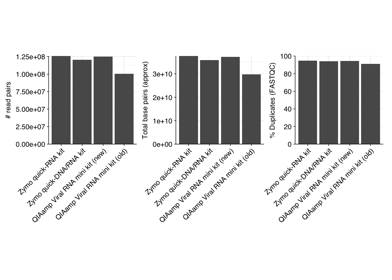
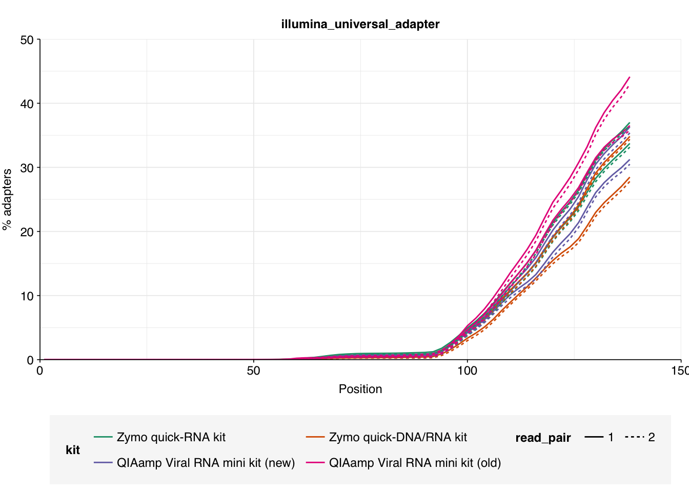
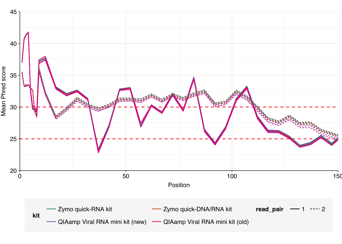
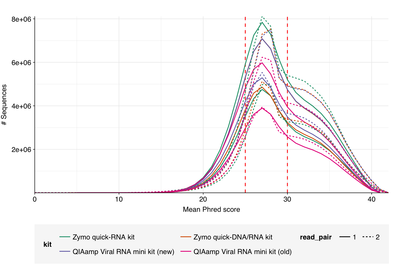
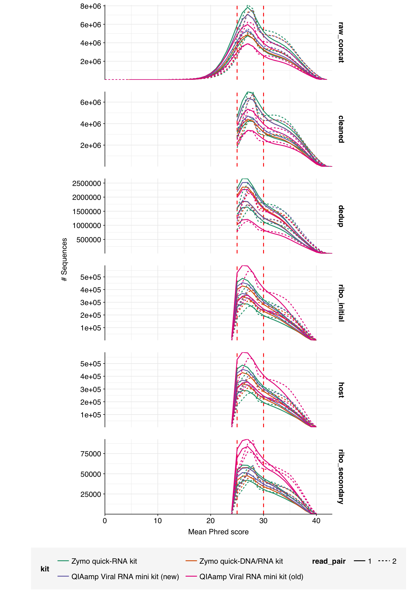
As before, we also got files containing “unmapped barcodes” reads that failed to be assigned to a sample; I ignored these as well. What remained consisted of roughly 470M read pairs, corresponding to roughly 140 Gb of sequencing data and distributed roughly evenly among the four sample groups. Reads were uniformly 150bp in length. Adapter levels were high, as were FASTQC-measured duplication levels. Quality levels were neither terrible nor great, but definitely worse than the previous DNA-seq data:
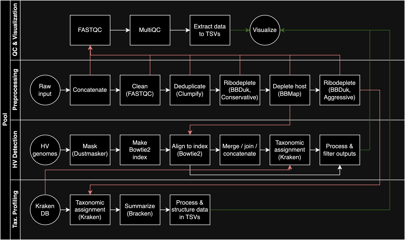
To process these data in an automated and reproducible manner, I created a Nextflow pipeline incorporating many of the steps I’ve discussed and looked into in previous notebooks. At the time of writing, the pipeline looks like this:
I start with preprocessing, including trimming, deduplication, and removal of host (human) and ribosomal sequences. The latter takes place in two stages, one conservative and the other aggressive. The output of conservative ribodepletion + host depletion is then forwarded to a human virus detection subpipeline via Bowtie2 and Kraken (more on that later), and the output of aggressive ribodepletion is then forwarded to a subpipeline for broader taxonomic profiling with Kraken and Bracken. The pipeline is still very much in progress, but the latest public version can be found here.
Preprocessing
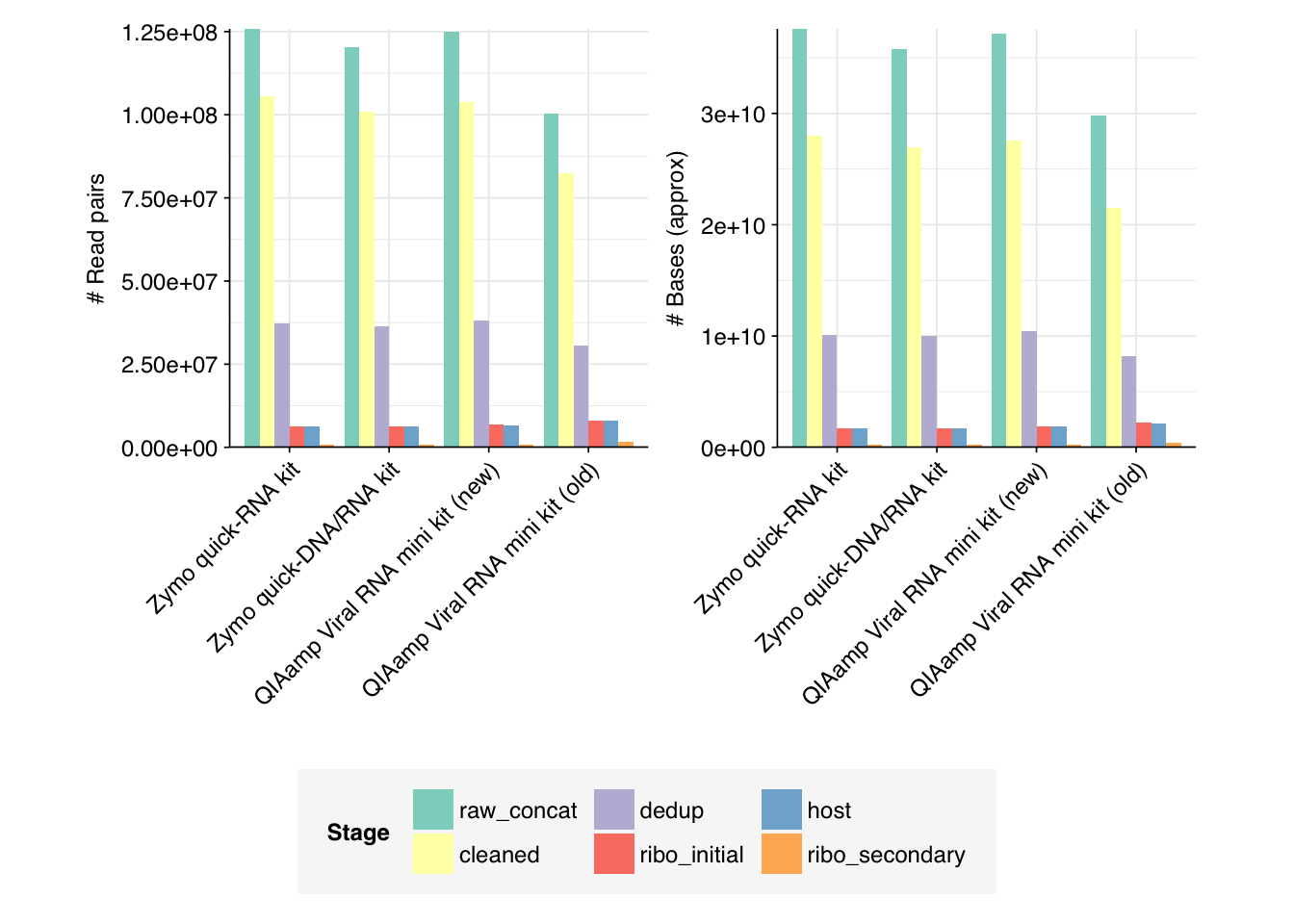
Very large read losses were observed during deduplication: cleaning, deduplication and conservative ribodepletion together removed about 94% of reads per sample, while host depletion and (primarily) secondary ribodepletion removed about 85% of the remainder, for an overall loss of 99%. A reasonable inference is that these samples contain a very high (98% or higher) fraction of ribosomal RNA, much higher than the ~20-50% seen in observation of past RNA-sequencing data. Our current main hypothesis is that this is the result of sequencing sludge rather than influent, but it could also be an effect of our protocols; head-to-head comparison of sludge and influent is needed to resolve this question.
Conversely, relatively few reads (25k to 50k per kit) were removed during host depletion. I actually suspect I’m being too conservative there and should loosen up parameters for future runs.
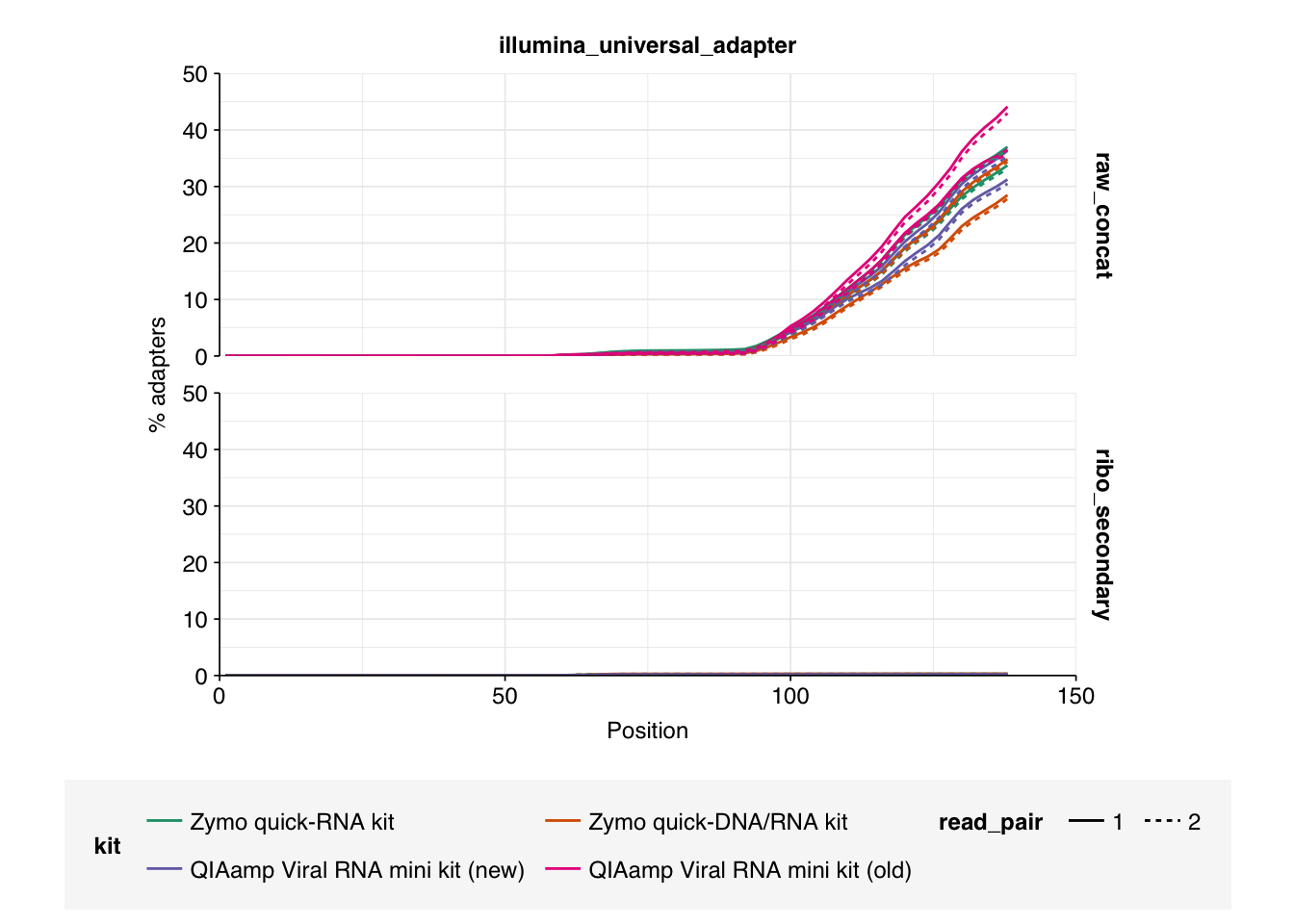
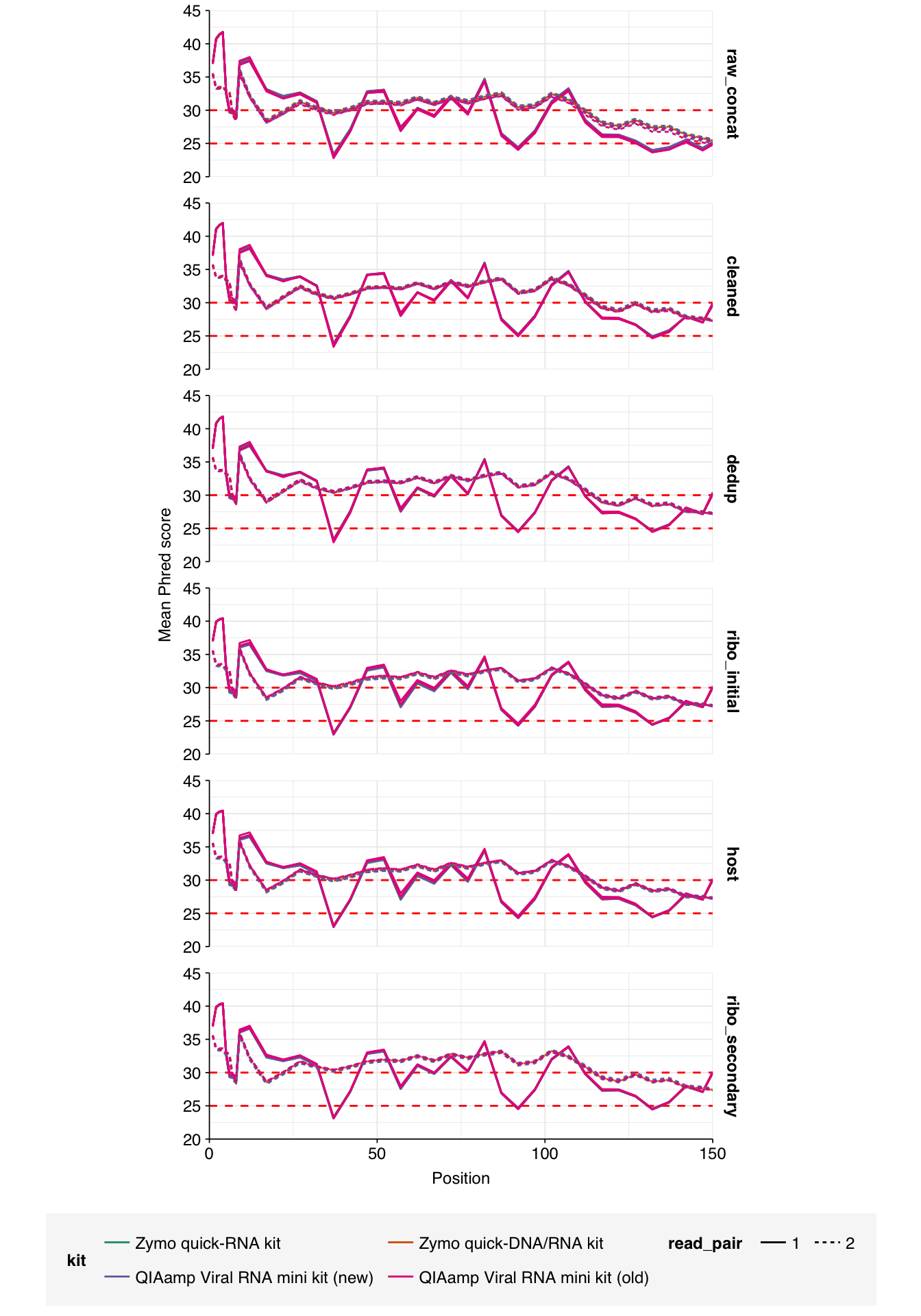
Data cleaning with FASTP was very successful at removing adapters, but only marginally successful at improving sequence quality; I might modify parameters to be more stringent on the latter front in future. Later stages in the pipeline had little effect on these factors.
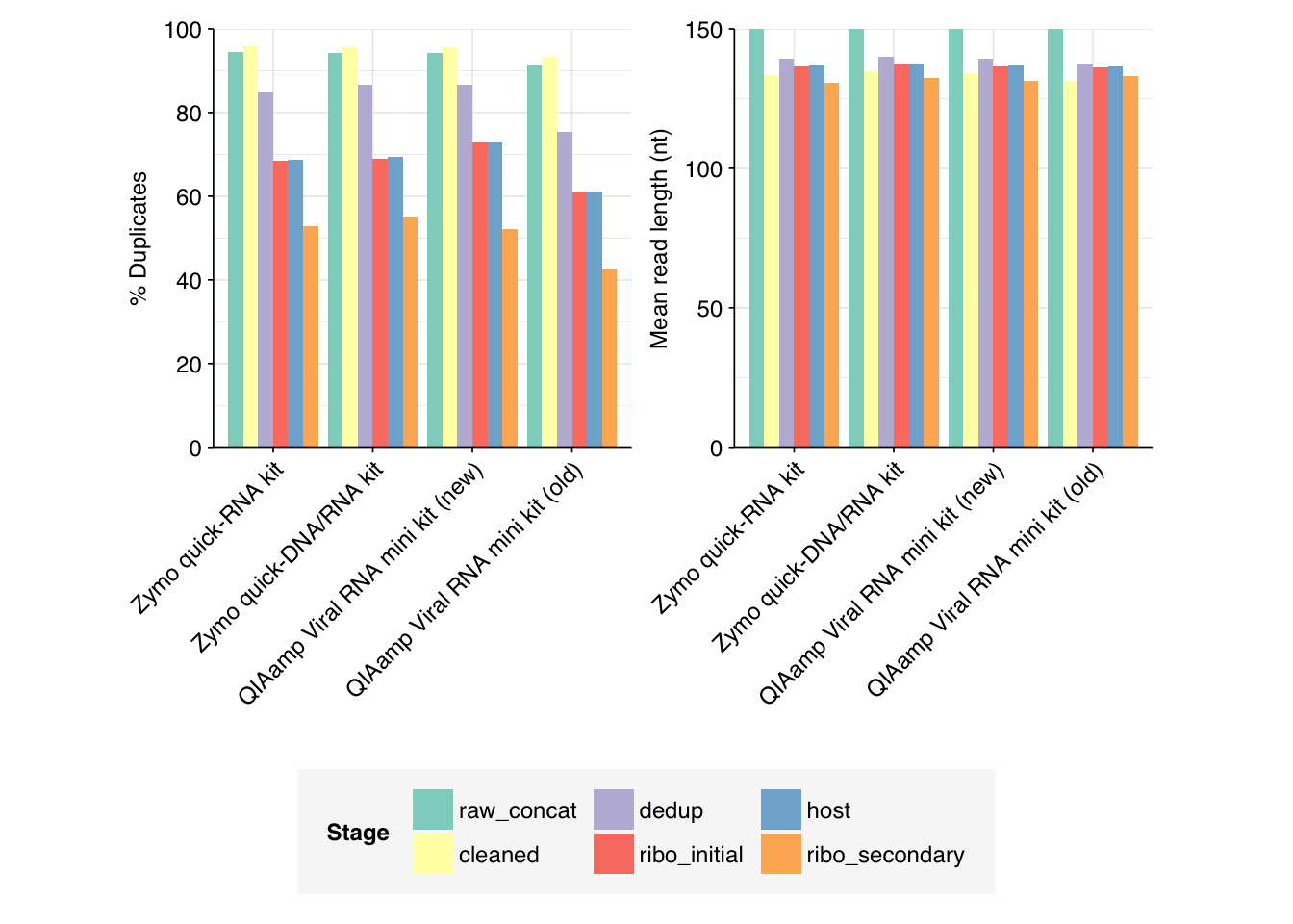
Duplicate levels as measured by FASTQC were only slightly reduced by deduplication with Clumpify. Ribodepletion achieved a significant further reduction in measured duplicate levels, suggesting that ribosomal sequences accounted for a disproportionate fraction of the surviving duplicates.
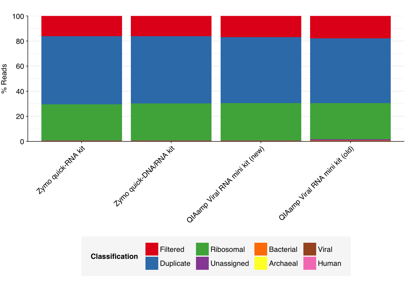
To assess the high-level composition of the reads, I ran the ribodepleted files through Kraken (using the Standard 16 database) and summarized the results with Bracken. Combining these results with the read counts above gives us a breakdown of the inferred composition of the samples:
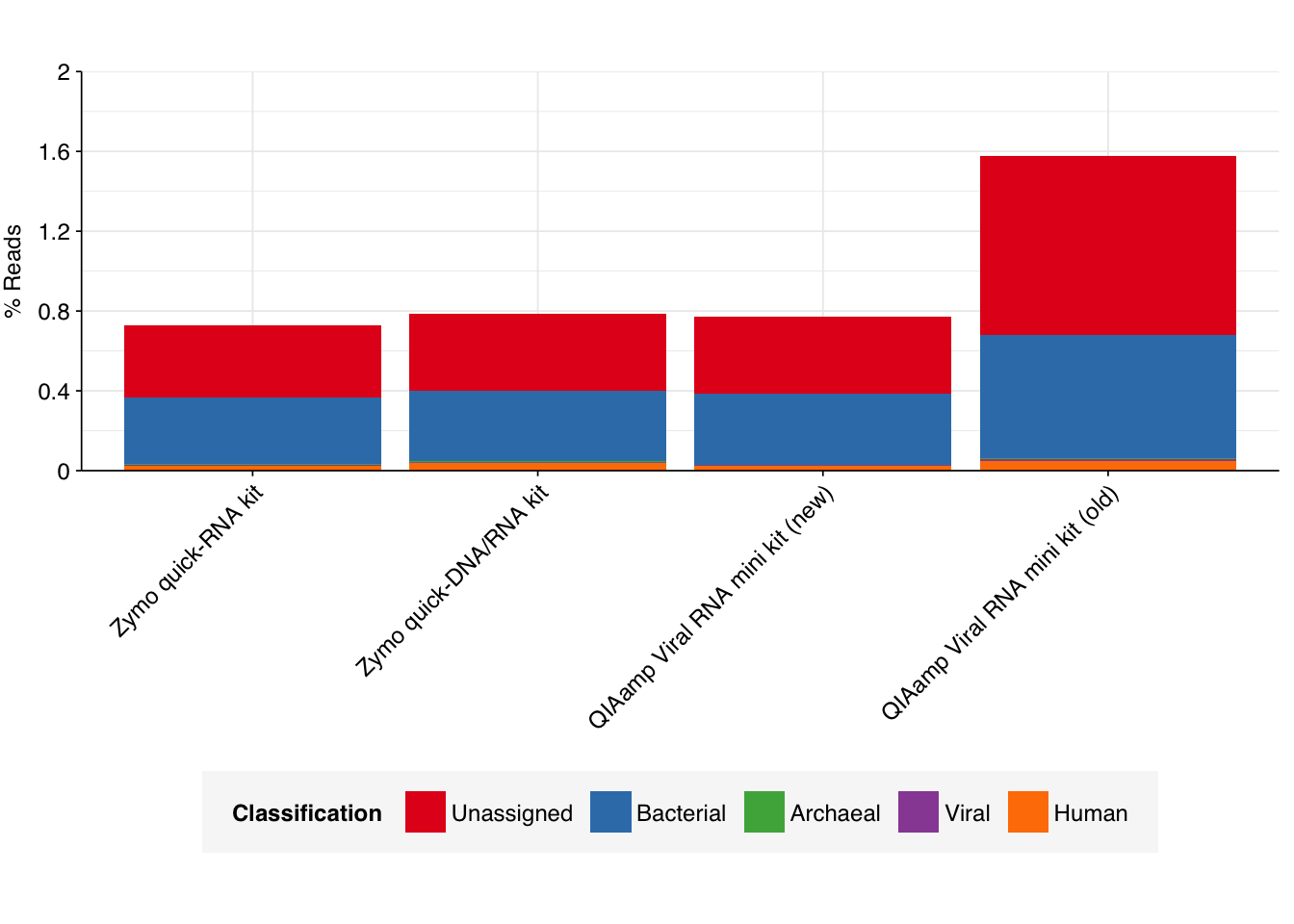
# Plot composition of minor componentsread_comp_minor<-read_comp_kits%>%filter(p_reads<0.1)g_comp_minor<-ggplot(read_comp_minor, aes(x=kit, y=p_reads, fill=classification))+geom_col(position ="stack")+scale_y_continuous(name ="% Reads", limits =c(0,0.02), breaks =seq(0,0.02,0.004), expand =c(0,0), labels =function(x)x*100)+scale_fill_brewer(palette ="Set1", name ="Classification")+theme_kit+theme(aspect.ratio =1/3)g_comp_minor
As we can see, nearly all the reads are removed during preprocessing as either low-quality, duplicates, or ribosomal. Of the remainder, most are either unclassified or bacterial. The fraction of human reads ranges from 0.2 to 0.5%, while the fraction of total viral reads ranges from 0.003 to 0.006%.
Human-viral reads, part 1: methods
To identify human-viral reads, I used a multi-stage process similar to the one outlined by Jeff in some of his past work. Specifically, after removing human reads with BBmap, the remaining reads went through the following steps:
Align reads to a database of human-infecting virus genomes with Bowtie2, with permissive parameters, & retain reads with at least one match. (Roughly 20k read pairs per kit, or 0.25% of all surviving non-host reads.)
Run reads that successfully align with Bowtie2 through Kraken2 (using the standard 16GB database) and exclude reads assigned by Kraken2 to any non-human-infecting-virus taxon. (Roughly 5500 surviving read pairs per kit.)
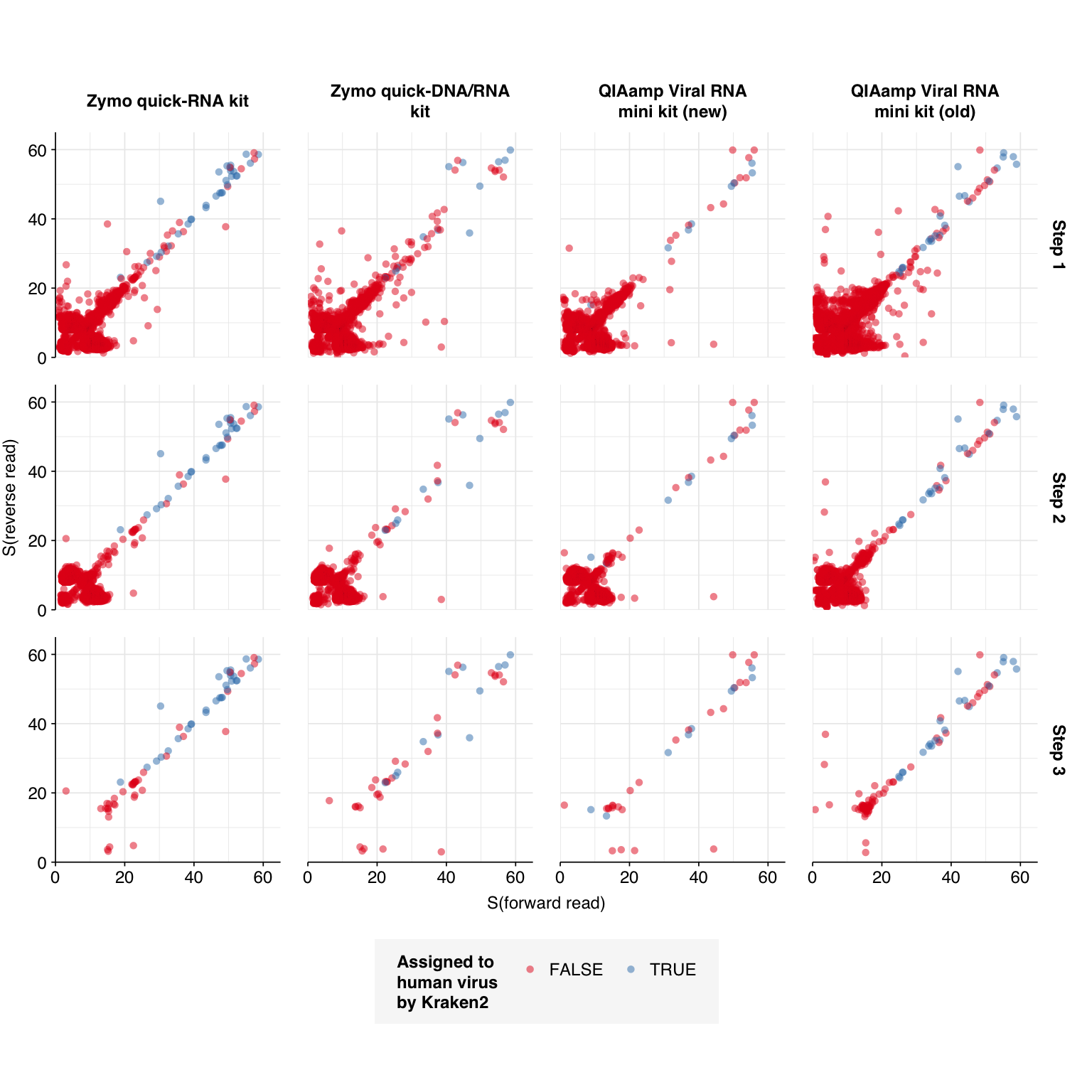
Calculate length-adjusted alignment score \(S=\frac{\text{bowtie2 alignment score}}{\ln(\text{read length})}\). Filter out reads that don’t meet at least one of the following four criteria:
The read pair is assigned to a human-infecting virus by both Kraken and Bowtie2
The read pair contains a Kraken2 hit to the same taxid as it is assigned to by Bowtie2.
The read pair is unassigned by Kraken and \(S>15\) for the forward read
The read pair is unassigned by Kraken and \(S>15\) for the reverse read
Applying all of these filtering steps leaves a total of 241 read pairs across all kits.
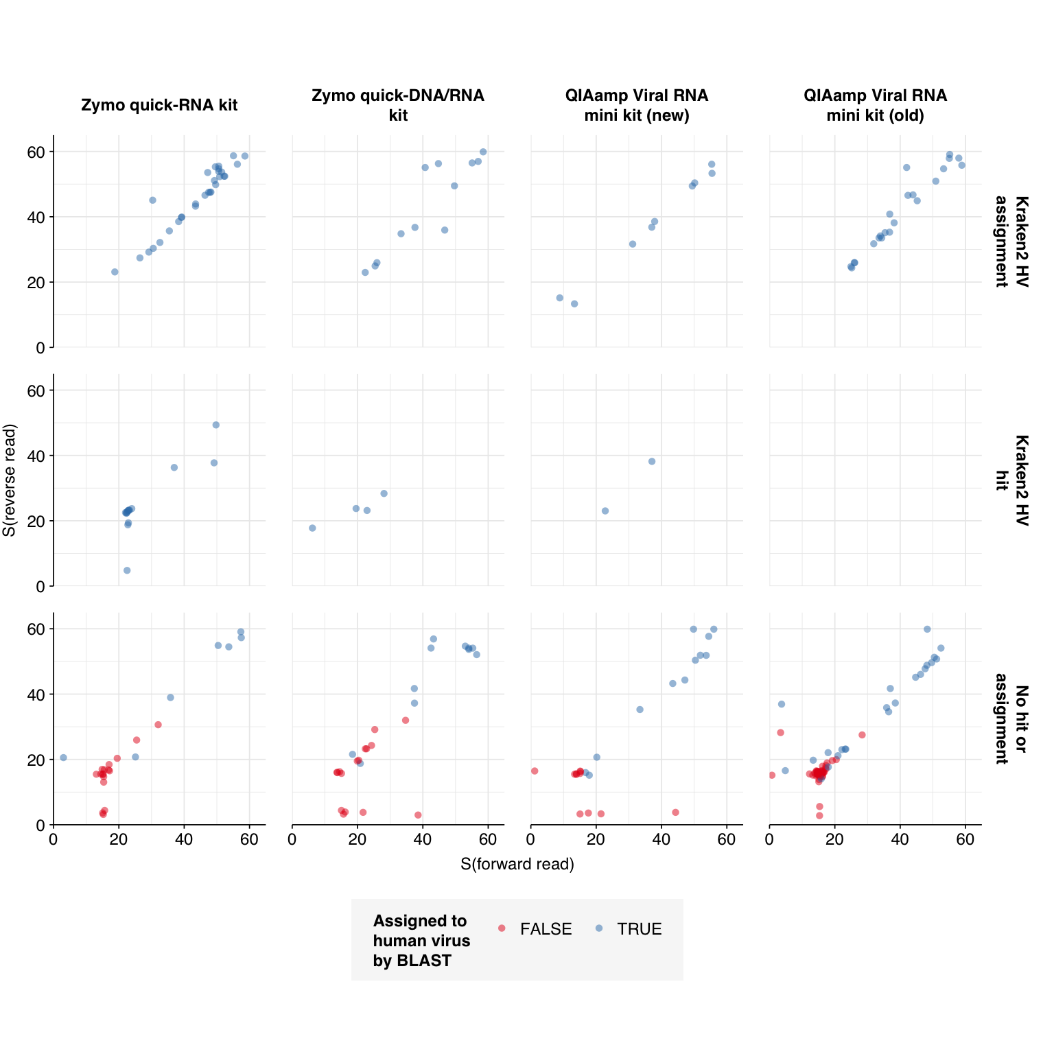
This was few enough that it was feasible for me to run all of them through NCBI BLAST (megablast against nt) and investigate which further filtering criteria give the best results in terms of sensitivity and specificity for human-infecting viruses:
As we can see, 100% of the reads that were marked as human-viral by both Kraken2 and Bowtie2 were also designated such by BLAST. Among reads not assigned by Kraken2, however, a lot of (mostly but not entirely low-scoring) read pairs that mapped to human viruses with Bowtie2 did not turn out to be viral when investigated manually.
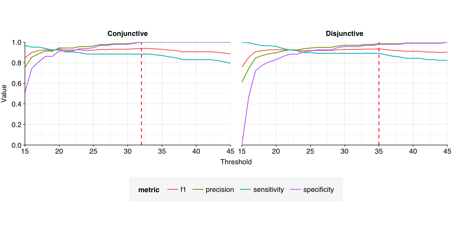
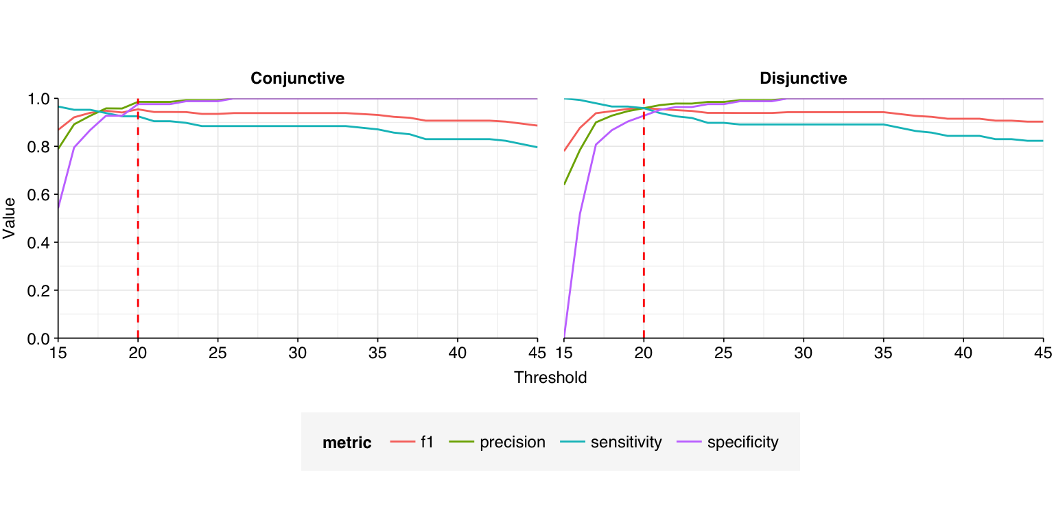
A natural approach to making overall HV read assignments would be to (1) accept reads that are assigned to HV by both Kraken2 and Bowtie2, and then (2) apply a length-normalised score threshold to reads that aren’t assigned to HV by Kraken. This threshold could either be conjunctive, requiring both the forward and reverse read to beat the threshold, or disjunctive, requiring only one or the other to do so. By treating the BLAST results as ground truth, we can evaluate what score threshold would provide the best overall method for identifying HV reads.
The red dashed lines indicate the threshold value with the highest F1 score (harmonic mean of precision and sensitivity), which is 32 for the conjunctive threshold and 35 for the disjunctive threshold. The disjunctive threshold achieves a slightly better F1 score (0.939 vs 0.936) – a fairly good score, but still worse than I’d ideally like for this use case.
Human-viral reads, part 2: cows?
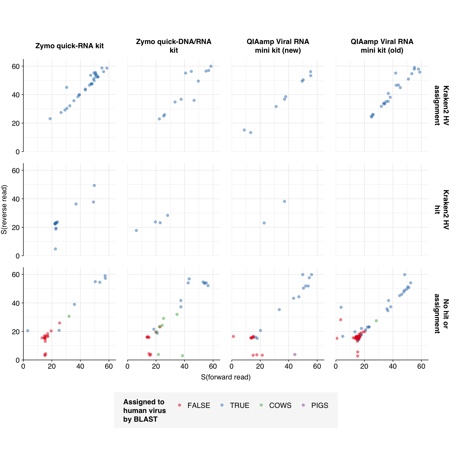
One odd pattern I noticed while doing the BLAST assignments was that a surprising number of read pairs were showing very strong alignment to bovine species (Bos taurus, Bos mutus, and relatives), as well as one showing strong alignment to pigs. These actually accounted for a pretty large fraction of high-scoring non-viral reads:
With the exception of one low-scoring read pair, all of the cow-mapping read pairs are unassigned by Kraken and mapped by Bowtie to the same taxon: Orf virus, a poxvirus that primarily infects livestock. BLAST will grudgingly find decent alignments to Orf virus for many of these reads if you restrict it to viral references, but alignments to bovine (and other ungulate) genomes show much better query coverage and % ID. Most of these reads appear to align well at many points in the bovine genome, across many different chromosomes, and none of them matched any conserved protein domains when I searched them on CD-search1. They also didn’t match any cow transposons when I searched on Dfam.
As such, I’m not really sure what these sequences are. That said, the idea of sequences from cows (and other mammalian livestock) getting into wastewater via human food (or directly via agriculture in some catchments) isn’t implausible.
If we remove these sequences from the dataset, we get a decent improvement in F1 score (>0.95) at a significantly lower score threshold:
As such, it seems worth trying to screen out cow and pig sequences prior to human virus read identification, in a similar manner to human sequences. I’ll look into adding this in the next version of the pipeline.
Human-viral reads, part 3: relative abundance
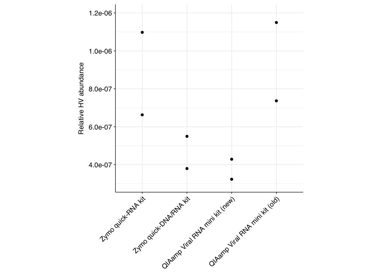
In the meantime, having done the BLAST verification, what can we say about overall abundance of human viruses in these samples?
Unsurprisingly, given the extremely high level of ribosomal sequences in these samples, the overall relative abundance of human viruses is quite low:
Among the three recent protocols, the Zymo quick-RNA achieves roughly double the mean relative HV abundance of the other kits. Comparing the two QIAamp protocols, the samples that didn’t undergo pre-extraction freezing also achieve more than double the relative HV abundance of those that did. It’s hard to know how much weight to put on these results, though, in the absence of replication.
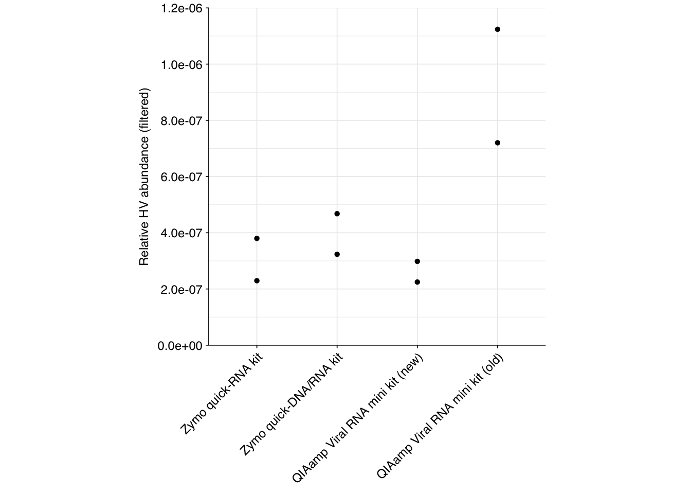
Counting up reads by target virus, we see that the most common target across all protocols is Influenza A virus (various strains), following by human picobirnavirus, mamastroviruses, and norovirus GII. The Zymo quick-RNA kit finds way more influenza A viruses than other kits, suggesting it may have some methodological advantage for some viruses:
However, in the DNA data from this BMC submission we previously observed contamination with Influenza A H3N2 segment 4 reads, which might also be affecting this run. Checking, it seems like a large fraction (but not all) of the flu-assigned reads mapping here do indeed align to H3N2 segment 4. Filtering out these likely-contaminant reads removes the apparent advantage of the Zymo quick-RNA kit, while retaining the high-performance of the non-freeze-thaw QIAamp protocol:
Based on the results of this analysis, I currently have the following next actions where this pipeline is concerned:
Experiment with making FASTP parameters more stringent to remove more low-quality reads.
Experiment with making BBMap parameters less stringent to remove more human reads.
Add additional filtering for cow and other mammalian livestock to preprocessing pipeline, and verify that this improves HV read identification.
Continue investigating alternative options for deduplication, especially removal of reverse-complement duplicates.
Continue working on implementing core pipeline functionality, including implementing a proper config file, reading and writing from AWS S3, running jobs through aws-batch, and investigating nf-core modules that could be integrated.
Try running this workflow on other available datasets and see how performance compares.
Footnotes
Though they might be too short; I don’t use CD-search enough to have a great sense of minimum length requirements.↩︎
Source Code
---title: "Workflow analysis of Project Runway RNA-seq testing data"subtitle: "Applying a new workflow to some oldish data."author: "Will Bradshaw"date: 2023-12-19format: html: code-fold: true code-tools: true code-link: true df-print: pagededitor: visualtitle-block-banner: black---```{r}#| label: load-packages#| include: falselibrary(tidyverse)library(cowplot)library(patchwork)library(fastqcr)source("../scripts/aux_plot-theme.R")theme_kit <- theme_base +theme(aspect.ratio =1,axis.text.x =element_text(hjust =1, angle =45),axis.title.x =element_blank())```On 2023-11-06, we received the RNA-sequencing portion of the testing data we ordered in late September, partner to the DNA data I analyzed in a previous notebook. At the time, I didn't do much in-depth analysis of these data, other than doing some basic QC and preprocessing and noting that the ribosomal fraction seemed very high. Now, having spent some time working on a new Nextflow workflow for analyzing sequencing data, I'm coming back to these data to apply that workflow and look at the results.# BackgroundAs before, we have raw sequencing data corresponding to nucleic-acid extractions from primary sludge samples from wastewater treatment plant A using three different extraction kits:- Zymo quick-RNA kit (kit 1)- Zymo quick-DNA/RNA kit (kit 2)- QIAamp Viral RNA mini kit (kit 6)For RNA-sequencing, we sent two DNase-treated replicates (A and C) to the BMC for each kit. We also sent two earlier sludge samples (denoted SS1 and SS2 here), processed with kit 6 via a slightly different protocol (in particular, without a freeze-thaw between concentration and extraction), for a total of eight samples. As before, these samples underwent library prep at the BMC followed by Element AVITI sequencing.# The raw dataThe raw data from the BMC in this case consisted of sixty-four FASTQ files, or eight per sample. Half of these were from an earlier failed sequencing run and contain little or no data; I ignored them. The other half were from the successful run. For some reason, each sample was processed as two libraries, each of which was added to both of the two lanes of the AVITI flow cell, for a total of four sequencing "samples" per input sample. For simplicity, I concatenated all four of these into one for downstream analysis.As before, we also got files containing "unmapped barcodes" reads that failed to be assigned to a sample; I ignored these as well. What remained consisted of roughly 470M read pairs, corresponding to roughly 140 Gb of sequencing data and distributed roughly evenly among the four sample groups. Reads were uniformly 150bp in length. Adapter levels were high, as were FASTQC-measured duplication levels. Quality levels were neither terrible nor great, but definitely worse than the previous DNA-seq data:```{r}# Import statskits <-tibble(sample =c("1A", "1C", "2A", "2C", "6A", "6C", "SS1", "SS2"),kit =c(rep("Zymo quick-RNA kit", 2),rep("Zymo quick-DNA/RNA kit", 2),rep("QIAamp Viral RNA mini kit (new)", 2),rep("QIAamp Viral RNA mini kit (old)", 2))) %>%mutate(kit =fct_inorder(kit))stages <-c("raw_concat", "cleaned", "dedup", "ribo_initial", "host", "ribo_secondary")data_dir <-"../data/2023-12-19_rna-seq-workflow/"basic_stats_path <-file.path(data_dir, "basic_stats.tsv")adapter_stats_path <-file.path(data_dir, "adapter_stats.tsv")quality_base_stats_path <-file.path(data_dir, "quality_base_stats.tsv")quality_seq_stats_path <-file.path(data_dir, "quality_sequence_stats.tsv")# Extract statsbasic_stats <-read_tsv(basic_stats_path, show_col_types =FALSE) %>%inner_join(kits, by="sample") %>%mutate(stage =factor(stage, levels = stages))adapter_stats <-read_tsv(adapter_stats_path, show_col_types =FALSE) %>%inner_join(kits, by="sample") %>%mutate(stage =factor(stage, levels = stages), read_pair =fct_inorder(as.character(read_pair)))quality_base_stats <-read_tsv(quality_base_stats_path, show_col_types =FALSE) %>%inner_join(kits, by="sample") %>%mutate(stage =factor(stage, levels = stages), read_pair =fct_inorder(as.character(read_pair)))quality_seq_stats <-read_tsv(quality_seq_stats_path, show_col_types =FALSE) %>%inner_join(kits, by="sample") %>%mutate(stage =factor(stage, levels = stages), read_pair =fct_inorder(as.character(read_pair)))# Filter to raw databasic_stats_raw <- basic_stats %>%filter(stage =="raw_concat") %>%group_by(kit) %>%summarize(n_read_pairs =sum(n_read_pairs), n_bases_approx =sum(n_bases_approx),percent_duplicates =mean(percent_duplicates), mean_seq_len =mean(mean_seq_len))adapter_stats_raw <- adapter_stats %>%filter(stage =="raw_concat")quality_base_stats_raw <- quality_base_stats %>%filter(stage =="raw_concat")quality_seq_stats_raw <- quality_seq_stats %>%filter(stage =="raw_concat")# Visualizeg_nreads_raw <-ggplot(basic_stats_raw, aes(x=kit, y=n_read_pairs)) +geom_col() +scale_y_continuous(name="# read pairs", expand=c(0,0)) + theme_base + theme_kitg_nbases_raw <-ggplot(basic_stats_raw, aes(x=kit, y=n_bases_approx)) +geom_col() +scale_y_continuous(name="Total base pairs (approx)", expand=c(0,0)) + theme_base + theme_kitg_ndup_raw <-ggplot(basic_stats_raw, aes(x=kit, y=percent_duplicates)) +geom_col() +scale_y_continuous(name="% Duplicates (FASTQC)", expand=c(0,0), limits =c(0,100), breaks =seq(0,100,20)) + theme_base + theme_kitg_adapters_raw <-ggplot(adapter_stats_raw,aes(x=position, y=pc_adapters, color=kit, linetype = read_pair, group=interaction(sample,read_pair))) +geom_line() +scale_color_brewer(palette ="Dark2") +scale_y_continuous(name="% adapters", limits=c(0,50),breaks =seq(0,100,10), expand=c(0,0)) +scale_x_continuous(name="Position", limits=c(0,150),breaks=seq(0,150,50), expand=c(0,0)) +guides(color=guide_legend(nrow=2,byrow=TRUE)) +facet_wrap(~adapter) + theme_baseg_quality_base_raw <-ggplot(quality_base_stats_raw,aes(x=position, y=mean_phred_score, color=kit, linetype = read_pair, group=interaction(sample,read_pair))) +geom_hline(yintercept=25, linetype="dashed", color="red") +geom_hline(yintercept=30, linetype="dashed", color="red") +geom_line() +scale_color_brewer(palette ="Dark2") +scale_y_continuous(name="Mean Phred score", expand=c(0,0), limits=c(20,45)) +scale_x_continuous(name="Position", limits=c(0,150),breaks=seq(0,150,50), expand=c(0,0)) +guides(color=guide_legend(nrow=2,byrow=TRUE)) + theme_baseg_quality_seq_raw <-ggplot(quality_seq_stats_raw,aes(x=mean_phred_score, y=n_sequences, color=kit, linetype = read_pair, group=interaction(sample,read_pair))) +geom_vline(xintercept=25, linetype="dashed", color="red") +geom_vline(xintercept=30, linetype="dashed", color="red") +geom_line() +scale_color_brewer(palette ="Dark2") +scale_x_continuous(name="Mean Phred score", expand=c(0,0)) +scale_y_continuous(name="# Sequences", expand=c(0,0)) +guides(color=guide_legend(nrow=2,byrow=TRUE)) + theme_baseg_nreads_raw + g_nbases_raw + g_ndup_rawg_adapters_rawg_quality_base_rawg_quality_seq_raw```# The pipelineTo process these data in an automated and reproducible manner, I created a Nextflow pipeline incorporating many of the steps I've discussed and looked into in previous notebooks. At the time of writing, the pipeline looks like this:{fig-align="center"}I start with preprocessing, including trimming, deduplication, and removal of host (human) and ribosomal sequences. The latter takes place in two stages, one conservative and the other aggressive. The output of conservative ribodepletion + host depletion is then forwarded to a human virus detection subpipeline via Bowtie2 and Kraken (more on that later), and the output of aggressive ribodepletion is then forwarded to a subpipeline for broader taxonomic profiling with Kraken and Bracken. The pipeline is still very much in progress, but the latest public version can be found [here](https://github.com/naobservatory/mgs-workflow).# PreprocessingVery large read losses were observed during deduplication: cleaning, deduplication and conservative ribodepletion together removed about 94% of reads per sample, while host depletion and (primarily) secondary ribodepletion removed about 85% of the remainder, for an overall loss of 99%. A reasonable inference is that these samples contain a very high (98% or higher) fraction of ribosomal RNA, much higher than the \~20-50% seen in observation of past RNA-sequencing data. Our current main hypothesis is that this is the result of sequencing sludge rather than influent, but it could also be an effect of our protocols; head-to-head comparison of sludge and influent is needed to resolve this question.```{r}basic_stats_stages <- basic_stats %>%group_by(kit,stage) %>%summarize(n_read_pairs =sum(n_read_pairs), n_bases_approx =sum(n_bases_approx), .groups ="drop", mean_seq_len =mean(mean_seq_len), percent_duplicates =mean(percent_duplicates))g_reads_stages <-ggplot(basic_stats_stages, aes(x=kit, y=n_read_pairs, fill=stage)) +geom_col(position="dodge") +scale_fill_brewer(palette ="Set3", name="Stage") +scale_y_continuous("# Read pairs", expand=c(0,0)) + theme_kitg_bases_stages <-ggplot(basic_stats_stages, aes(x=kit, y=n_bases_approx, fill=stage)) +geom_col(position="dodge") +scale_fill_brewer(palette ="Set3", name="Stage") +scale_y_continuous("# Bases (approx)", expand=c(0,0)) + theme_kitlegend <-get_legend(g_reads_stages)tnl <-theme(legend.position ="none")plot_grid((g_reads_stages + tnl) + (g_bases_stages + tnl), legend, nrow =2,rel_heights =c(4,1))```Conversely, relatively few reads (25k to 50k per kit) were removed during host depletion. I actually suspect I'm being too conservative there and should loosen up parameters for future runs.Data cleaning with FASTP was very successful at removing adapters, but only marginally successful at improving sequence quality; I might modify parameters to be more stringent on the latter front in future. Later stages in the pipeline had little effect on these factors.```{r}# Per-stage adapter contentg_adapters_stages <-ggplot(adapter_stats,aes(x=position, y=pc_adapters, color=kit, linetype = read_pair, group=interaction(sample,read_pair))) +geom_line() +scale_color_brewer(palette ="Dark2") +scale_y_continuous(name="% adapters", limits=c(0,50),breaks =seq(0,100,10), expand=c(0,0)) +scale_x_continuous(name="Position", limits=c(0,150),breaks=seq(0,150,50), expand=c(0,0)) +guides(color=guide_legend(nrow=2,byrow=TRUE)) +facet_grid(stage~adapter) + theme_base +theme(aspect.ratio =0.33)g_adapters_stages``````{r}#| fig-height: 10# Per-stage quality metricsg_quality_base_stages <-ggplot(quality_base_stats,aes(x=position, y=mean_phred_score, color=kit, linetype = read_pair, group=interaction(sample,read_pair))) +geom_hline(yintercept=25, linetype="dashed", color="red") +geom_hline(yintercept=30, linetype="dashed", color="red") +geom_line() +scale_color_brewer(palette ="Dark2") +scale_y_continuous(name="Mean Phred score", expand=c(0,0), limits=c(20,45)) +scale_x_continuous(name="Position", limits=c(0,150),breaks=seq(0,150,50), expand=c(0,0)) +guides(color=guide_legend(nrow=2,byrow=TRUE)) +facet_grid(stage~.) + theme_base +theme(aspect.ratio =0.33)g_quality_seq_stages <-ggplot(quality_seq_stats,aes(x=mean_phred_score, y=n_sequences, color=kit, linetype = read_pair, group=interaction(sample,read_pair))) +geom_vline(xintercept=25, linetype="dashed", color="red") +geom_vline(xintercept=30, linetype="dashed", color="red") +geom_line() +scale_color_brewer(palette ="Dark2") +scale_x_continuous(name="Mean Phred score", expand=c(0,0)) +scale_y_continuous(name="# Sequences", expand=c(0,0)) +guides(color=guide_legend(nrow=2,byrow=TRUE)) +facet_grid(stage~., scales="free_y") + theme_base +theme(aspect.ratio =0.33)g_quality_base_stagesg_quality_seq_stages```Duplicate levels as measured by FASTQC were only slightly reduced by deduplication with Clumpify. Ribodepletion achieved a significant further reduction in measured duplicate levels, suggesting that ribosomal sequences accounted for a disproportionate fraction of the surviving duplicates.```{r}g_dup_stages <-ggplot(basic_stats_stages, aes(x=kit, y=percent_duplicates, fill=stage)) +geom_col(position="dodge") +scale_fill_brewer(palette ="Set3", name="Stage") +scale_y_continuous("% Duplicates", limits=c(0,100), breaks=seq(0,100,20), expand=c(0,0)) + theme_kitg_readlen_stages <-ggplot(basic_stats_stages, aes(x=kit, y=mean_seq_len, fill=stage)) +geom_col(position="dodge") +scale_fill_brewer(palette ="Set3", name="Stage") +scale_y_continuous("Mean read length (nt)", expand=c(0,0)) + theme_kitplot_grid((g_dup_stages + tnl) + (g_readlen_stages + tnl), legend, nrow =2,rel_heights =c(4,1))```# High-level compositionTo assess the high-level composition of the reads, I ran the ribodepleted files through Kraken (using the Standard 16 database) and summarized the results with Bracken. Combining these results with the read counts above gives us a breakdown of the inferred composition of the samples:```{r}# Import Bracken databracken_path <-file.path(data_dir, "bracken_counts.tsv")bracken <-read_tsv(bracken_path, show_col_types =FALSE)total_assigned <- bracken %>%group_by(sample) %>%summarize(name ="Total",kraken_assigned_reads =sum(kraken_assigned_reads),added_reads =sum(added_reads),new_est_reads =sum(new_est_reads),fraction_total_reads =sum(fraction_total_reads))bracken_spread <- bracken %>%select(name, sample, new_est_reads) %>%mutate(name =tolower(name)) %>%pivot_wider(id_cols ="sample", names_from ="name", values_from ="new_est_reads")# Count readsread_counts_preproc <- basic_stats %>%select(kit, sample, stage, n_read_pairs) %>%pivot_wider(id_cols =c("kit", "sample"), names_from="stage", values_from="n_read_pairs")read_counts <- read_counts_preproc %>%inner_join(total_assigned %>%select(sample, new_est_reads), by ="sample") %>%rename(assigned = new_est_reads) %>%inner_join(bracken_spread, by="sample")# Assess compositionread_comp <-transmute(read_counts, kit=kit, sample=sample,n_filtered = raw_concat-cleaned,n_duplicate = cleaned-dedup,n_ribosomal = (dedup-ribo_initial) + (host-ribo_secondary),n_unassigned = ribo_secondary-assigned,n_bacterial = bacteria,n_archaeal = archaea,n_viral = viruses,n_human = (ribo_initial-host) + eukaryota)read_comp_long <-pivot_longer(read_comp, -(kit:sample), names_to ="classification",names_prefix ="n_", values_to ="n_reads") %>%mutate(classification =fct_inorder(str_to_sentence(classification))) %>%group_by(sample) %>%mutate(p_reads = n_reads/sum(n_reads))read_comp_kits <- read_comp_long %>%group_by(kit, classification) %>%summarize(n_reads =sum(n_reads), .groups ="drop") %>%group_by(kit) %>%mutate(p_reads = n_reads/sum(n_reads))# Plot overall compositiong_comp <-ggplot(read_comp_kits, aes(x=kit, y=p_reads, fill=classification)) +geom_col(position ="stack") +scale_y_continuous(name ="% Reads", limits =c(0,1), breaks =seq(0,1,0.2),expand =c(0,0), labels =function(x) x*100) +scale_fill_brewer(palette ="Set1", name ="Classification") + theme_kit +theme(aspect.ratio =1/3)g_comp# Plot composition of minor componentsread_comp_minor <- read_comp_kits %>%filter(p_reads <0.1)g_comp_minor <-ggplot(read_comp_minor, aes(x=kit, y=p_reads, fill=classification)) +geom_col(position ="stack") +scale_y_continuous(name ="% Reads", limits =c(0,0.02), breaks =seq(0,0.02,0.004),expand =c(0,0), labels =function(x) x*100) +scale_fill_brewer(palette ="Set1", name ="Classification") + theme_kit +theme(aspect.ratio =1/3)g_comp_minor```As we can see, nearly all the reads are removed during preprocessing as either low-quality, duplicates, or ribosomal. Of the remainder, most are either unclassified or bacterial. The fraction of human reads ranges from 0.2 to 0.5%, while the fraction of total viral reads ranges from 0.003 to 0.006%.# Human-viral reads, part 1: methodsTo identify human-viral reads, I used a multi-stage process similar to the one outlined by Jeff in some of his past work. Specifically, after removing human reads with BBmap, the remaining reads went through the following steps:1. Align reads to a database of human-infecting virus genomes with Bowtie2, with permissive parameters, & retain reads with at least one match. (Roughly 20k read pairs per kit, or 0.25% of all surviving non-host reads.)2. Run reads that successfully align with Bowtie2 through Kraken2 (using the standard 16GB database) and exclude reads assigned by Kraken2 to any non-human-infecting-virus taxon. (Roughly 5500 surviving read pairs per kit.)3. Calculate length-adjusted alignment score $S=\frac{\text{bowtie2 alignment score}}{\ln(\text{read length})}$. Filter out reads that don't meet at least one of the following four criteria: - The read pair is *assigned* to a human-infecting virus by both Kraken and Bowtie2 - The read pair contains a Kraken2 *hit* to the same taxid as it is assigned to by Bowtie2. - The read pair is unassigned by Kraken and $S>15$ for the forward read - The read pair is unassigned by Kraken and $S>15$ for the reverse readApplying all of these filtering steps leaves a total of 241 read pairs across all kits.```{r}#| warning: false#| fig-width: 8#| fig-height: 8# Import Bowtie2/Kraken data and perform filtering stepsmrg_path <-file.path(data_dir, "hv_hits_putative.tsv")mrg0 <-read_tsv(mrg_path, show_col_types =FALSE) %>%inner_join(kits, by="sample") %>%mutate(filter_step=1) %>%select(kit, sample, seq_id, taxid, assigned_taxid, adj_score_fwd, adj_score_rev, classified, assigned_hv, query_seq_fwd, query_seq_rev, encoded_hits, filter_step) %>%arrange(sample, desc(adj_score_fwd), desc(adj_score_rev))mrg1 <- mrg0 %>%filter((!classified) | assigned_hv) %>%mutate(filter_step=2)mrg2 <- mrg1 %>%mutate(hit_hv =!is.na(str_match(encoded_hits, paste0(" ", as.character(taxid), ":")))) %>%filter(adj_score_fwd >15| adj_score_rev >15| assigned_hv | hit_hv) %>%mutate(filter_step=3)mrg_all <-bind_rows(mrg0, mrg1, mrg2)# Visualizeg_mrg <-ggplot(mrg_all, aes(x=adj_score_fwd, y=adj_score_rev, color=assigned_hv)) +geom_point(alpha=0.5, shape=16) +scale_color_brewer(palette="Set1", name="Assigned to\nhuman virus\nby Kraken2") +scale_x_continuous(name="S(forward read)", limits=c(0,65), breaks=seq(0,100,20), expand =c(0,0)) +scale_y_continuous(name="S(reverse read)", limits=c(0,65), breaks=seq(0,100,20), expand =c(0,0)) +facet_grid(filter_step~kit, labeller =labeller(filter_step=function(x) paste("Step", x), kit =label_wrap_gen(20))) + theme_base +theme(aspect.ratio=1)g_mrg```This was few enough that it was feasible for me to run all of them through NCBI BLAST (megablast against nt) and investigate which further filtering criteria give the best results in terms of sensitivity and specificity for human-infecting viruses:```{r}#| warning: false#| fig-width: 8#| fig-height: 8hv_blast <-list(`1A`=c(rep(TRUE, 40), TRUE, TRUE, TRUE, FALSE, FALSE, FALSE, FALSE, FALSE, FALSE, TRUE),`1C`=c(rep(TRUE, 5), "COWS", TRUE, TRUE, FALSE, TRUE, rep(FALSE, 9)),`2A`=c(rep(TRUE, 10), "COWS", TRUE, "COWS", "COWS", TRUE,FALSE, "COWS", FALSE, TRUE, TRUE,FALSE, FALSE, FALSE, FALSE, TRUE),`2C`=c(rep(TRUE, 5), TRUE, "COWS", TRUE, TRUE, TRUE, TRUE, TRUE, "COWS", TRUE, "COWS", FALSE, FALSE, FALSE), `6A`=c(rep(TRUE, 10), FALSE, TRUE, FALSE, FALSE, FALSE, FALSE, TRUE, TRUE, FALSE), `6C`=c(rep(TRUE, 5), "PIGS", TRUE, TRUE, TRUE, TRUE,FALSE, TRUE, FALSE, FALSE, FALSE), SS1 =c(rep(TRUE, 5), rep(FALSE, 10),"FALSE", "COWS", "FALSE", "FALSE", "FALSE",rep(FALSE, 15) ),SS2 =c(rep(TRUE, 25), TRUE, "COWS", TRUE, TRUE, TRUE,TRUE, TRUE, TRUE, TRUE, TRUE,FALSE, TRUE, TRUE, FALSE, FALSE,FALSE, FALSE, TRUE, FALSE, FALSE,rep(FALSE, 5),FALSE, FALSE, FALSE, FALSE, TRUE,FALSE, FALSE, TRUE, TRUE, FALSE) )mrg3 <- mrg2 %>%group_by(sample) %>%mutate(seq_num =row_number()) %>% ungroup %>%mutate(hv_blast =unlist(hv_blast),kraken_label =ifelse(assigned_hv, "Kraken2 HV\nassignment",ifelse(hit_hv, "Kraken2 HV\nhit","No hit or\nassignment")))g_mrg3_1 <- mrg3 %>%mutate(hv_blast = hv_blast =="TRUE") %>%ggplot(aes(x=adj_score_fwd, y=adj_score_rev, color=hv_blast)) +geom_point(alpha=0.5, shape=16) +scale_color_brewer(palette="Set1", name="Assigned to\nhuman virus\nby BLAST") +scale_x_continuous(name="S(forward read)", limits=c(0,65), breaks=seq(0,100,20), expand =c(0,0)) +scale_y_continuous(name="S(reverse read)", limits=c(0,65), breaks=seq(0,100,20), expand =c(0,0)) +facet_grid(kraken_label~kit, labeller =labeller(kit =label_wrap_gen(20))) + theme_base +theme(aspect.ratio=1)g_mrg3_1```As we can see, 100% of the reads that were marked as human-viral by both Kraken2 and Bowtie2 were also designated such by BLAST. Among reads not assigned by Kraken2, however, a lot of (mostly but not entirely low-scoring) read pairs that mapped to human viruses with Bowtie2 did not turn out to be viral when investigated manually.A natural approach to making overall HV read assignments would be to (1) accept reads that are assigned to HV by both Kraken2 and Bowtie2, and then (2) apply a length-normalised score threshold to reads that aren't assigned to HV by Kraken. This threshold could either be conjunctive, requiring both the forward and reverse read to beat the threshold, or disjunctive, requiring only one or the other to do so. By treating the BLAST results as ground truth, we can evaluate what score threshold would provide the best overall method for identifying HV reads.```{r}#| fig-width: 8#| fig-height: 4# Test sensitivity and specificitytest_sens_spec <-function(tab, score_threshold, conjunctive, include_special){if (!include_special) tab <-filter(tab, hv_blast %in%c("TRUE", "FALSE")) tab_retained <- tab %>%mutate(conjunctive = conjunctive,retain_score_conjunctive = (adj_score_fwd > score_threshold & adj_score_rev > score_threshold), retain_score_disjunctive = (adj_score_fwd > score_threshold | adj_score_rev > score_threshold),retain_score =ifelse(conjunctive, retain_score_conjunctive, retain_score_disjunctive),retain = assigned_hv | hit_hv | retain_score) %>%group_by(hv_blast, retain) %>% count pos_tru <- tab_retained %>%filter(hv_blast =="TRUE", retain) %>%pull(n) %>% sum pos_fls <- tab_retained %>%filter(hv_blast !="TRUE", retain) %>%pull(n) %>% sum neg_tru <- tab_retained %>%filter(hv_blast !="TRUE", !retain) %>%pull(n) %>% sum neg_fls <- tab_retained %>%filter(hv_blast =="TRUE", !retain) %>%pull(n) %>% sum sensitivity <- pos_tru / (pos_tru + neg_fls) specificity <- neg_tru / (neg_tru + pos_fls) precision <- pos_tru / (pos_tru + pos_fls) f1 <-2* precision * sensitivity / (precision + sensitivity) out <-tibble(threshold=score_threshold, include_special = include_special, conjunctive = conjunctive, sensitivity=sensitivity, specificity=specificity, precision=precision, f1=f1)return(out)}stats_withcow_conj <-lapply(15:45, test_sens_spec, tab=mrg3, include_special=TRUE, conjunctive=TRUE) %>% bind_rowsstats_withcow_disj <-lapply(15:45, test_sens_spec, tab=mrg3, include_special=TRUE, conjunctive=FALSE) %>% bind_rowsstats_withcow <-bind_rows(stats_withcow_conj, stats_withcow_disj) %>%pivot_longer(!(threshold:conjunctive), names_to="metric", values_to="value") %>%mutate(conj_label =ifelse(conjunctive, "Conjunctive", "Disjunctive"))threshold_opt_withcow <- stats_withcow %>%group_by(conj_label) %>%filter(metric =="f1") %>%filter(value ==max(value)) %>%filter(threshold ==min(threshold))g_stats_withcow <-ggplot(stats_withcow, aes(x=threshold, y=value, color=metric)) +geom_line() +geom_vline(data = threshold_opt_withcow, mapping=aes(xintercept=threshold), color="red",linetype ="dashed") +scale_y_continuous(name ="Value", limits=c(0,1), breaks =seq(0,1,0.2), expand =c(0,0)) +scale_x_continuous(name ="Threshold", expand =c(0,0)) +facet_wrap(~conj_label) + theme_baseg_stats_withcow```The red dashed lines indicate the threshold value with the highest F1 score (harmonic mean of precision and sensitivity), which is 32 for the conjunctive threshold and 35 for the disjunctive threshold. The disjunctive threshold achieves a slightly better F1 score (0.939 vs 0.936) -- a fairly good score, but still worse than I'd ideally like for this use case.# Human-viral reads, part 2: cows?One odd pattern I noticed while doing the BLAST assignments was that a surprising number of read pairs were showing very strong alignment to bovine species (*Bos taurus, Bos mutus,* and relatives), as well as one showing strong alignment to pigs. These actually accounted for a pretty large fraction of high-scoring non-viral reads:```{r}#| warning: false#| fig-width: 8#| fig-height: 8g_mrg3_2 <- mrg3 %>%mutate(hv_blast =factor(hv_blast, levels =c("FALSE", "TRUE", "COWS", "PIGS"))) %>%ggplot(aes(x=adj_score_fwd, y=adj_score_rev, color=hv_blast)) +geom_point(alpha=0.5, shape=16) +scale_color_brewer(palette="Set1", name="Assigned to\nhuman virus\nby BLAST") +scale_x_continuous(name="S(forward read)", limits=c(0,65), breaks=seq(0,100,20), expand =c(0,0)) +scale_y_continuous(name="S(reverse read)", limits=c(0,65), breaks=seq(0,100,20), expand =c(0,0)) +facet_grid(kraken_label~kit, labeller =labeller(kit =label_wrap_gen(20))) + theme_base +theme(aspect.ratio=1)g_mrg3_2```With the exception of one low-scoring read pair, all of the cow-mapping read pairs are unassigned by Kraken and mapped by Bowtie to the same taxon: [Orf virus](https://en.wikipedia.org/wiki/Orf_(disease)), a poxvirus that primarily infects livestock. BLAST will grudgingly find decent alignments to Orf virus for many of these reads if you restrict it to viral references, but alignments to bovine (and other ungulate) genomes show much better query coverage and % ID. Most of these reads appear to align well at many points in the bovine genome, across many different chromosomes, and none of them matched any conserved protein domains when I searched them on CD-search[^1]. They also didn't match any cow transposons when I searched on Dfam.[^1]: Though they might be too short; I don't use CD-search enough to have a great sense of minimum length requirements.As such, I'm not really sure what these sequences are. That said, the idea of sequences from cows (and other mammalian livestock) getting into wastewater via human food (or directly via agriculture in some catchments) isn't implausible.If we remove these sequences from the dataset, we get a decent improvement in F1 score (\>0.95) at a significantly lower score threshold:```{r}#| fig-width: 8#| fig-height: 4stats_nocow_conj <-lapply(15:45, test_sens_spec, tab=mrg3, include_special=FALSE, conjunctive=TRUE) %>% bind_rowsstats_nocow_disj <-lapply(15:45, test_sens_spec, tab=mrg3, include_special=FALSE, conjunctive=FALSE) %>% bind_rowsstats_nocow <-bind_rows(stats_nocow_conj, stats_nocow_disj) %>%pivot_longer(!(threshold:conjunctive), names_to="metric", values_to="value") %>%mutate(conj_label =ifelse(conjunctive, "Conjunctive", "Disjunctive"))threshold_opt_nocow <- stats_nocow %>%group_by(conj_label) %>%filter(metric =="f1") %>%filter(value ==max(value)) %>%filter(threshold ==min(threshold))g_stats_nocow <-ggplot(stats_nocow, aes(x=threshold, y=value, color=metric)) +geom_line() +geom_vline(data = threshold_opt_nocow, mapping=aes(xintercept=threshold), color="red",linetype ="dashed") +scale_y_continuous(name ="Value", limits=c(0,1), breaks =seq(0,1,0.2), expand =c(0,0)) +scale_x_continuous(name ="Threshold", expand =c(0,0)) +facet_wrap(~conj_label) + theme_baseg_stats_nocow```As such, it seems worth trying to screen out cow and pig sequences prior to human virus read identification, in a similar manner to human sequences. I'll look into adding this in the next version of the pipeline.# Human-viral reads, part 3: relative abundanceIn the meantime, having done the BLAST verification, what can we say about overall abundance of human viruses in these samples?Unsurprisingly, given the extremely high level of ribosomal sequences in these samples, the overall relative abundance of human viruses is quite low:```{r}n_reads_hv <- mrg3 %>%filter(hv_blast =="TRUE") %>%group_by(kit) %>% count %>%rename(n_reads_hv = n)hv_abundance <-inner_join(basic_stats %>%filter(stage =="raw_concat"), n_reads_hv, by="kit") %>%mutate(hv_abundance = n_reads_hv/n_read_pairs)g_hv_abundance <-ggplot(hv_abundance, aes(x=kit, y=hv_abundance)) +geom_point(shape=16) +scale_y_continuous(name ="Relative HV abundance", limits=c(3e-7,1.2e-6),breaks =seq(2e-7, 1.2e-6, 2e-7)) + theme_kitg_hv_abundance```Among the three recent protocols, the Zymo quick-RNA achieves roughly double the mean relative HV abundance of the other kits. Comparing the two QIAamp protocols, the samples that didn't undergo pre-extraction freezing also achieve more than double the relative HV abundance of those that did. It's hard to know how much weight to put on these results, though, in the absence of replication.Counting up reads by target virus, we see that the most common target across all protocols is Influenza A virus (various strains), following by human picobirnavirus, mamastroviruses, and norovirus GII. The Zymo quick-RNA kit finds way more influenza A viruses than other kits, suggesting it may have some methodological advantage for some viruses:```{r}human_virus_path <-file.path(data_dir, "human-viruses.tsv")virus_names_path <-file.path(data_dir, "virus-names-short.txt")human_viruses <-read_tsv(human_virus_path, show_col_types =FALSE,col_names =c("taxid", "virus_name"),col_types =c("d", "c"))virus_names_short <-read_tsv(virus_names_path, show_col_types =FALSE)mrg4 <- mrg3 %>%filter(hv_blast =="TRUE") %>%inner_join(human_viruses, by="taxid") %>%inner_join(virus_names_short, by ="virus_name")virus_counts_total <- mrg4 %>%group_by(virus_name_short) %>%count(name="virus_count")virus_counts <- mrg4 %>%group_by(kit, virus_name_short) %>%count(name="virus_count") %>%pivot_wider(id_cols ="virus_name_short", names_from ="kit", values_from ="virus_count",values_fill =0) %>%inner_join(virus_counts_total, by="virus_name_short") %>%rename(Total = virus_count) %>%select(virus_name_short, Total, everything()) %>%arrange(desc(Total))virus_counts```However, in the DNA data from this BMC submission we previously observed contamination with Influenza A H3N2 segment 4 reads, which might also be affecting this run. Checking, it seems like a large fraction (but not all) of the flu-assigned reads mapping here do indeed align to H3N2 segment 4. Filtering out these likely-contaminant reads removes the apparent advantage of the Zymo quick-RNA kit, while retaining the high-performance of the non-freeze-thaw QIAamp protocol:```{r}flu_path <-file.path(data_dir, "flu-reads.tsv")flu <-read_tsv(flu_path, show_col_types =FALSE)n_reads_hv_filtered <- mrg3 %>%filter(hv_blast =="TRUE") %>%full_join(flu, by=c("sample", "seq_num")) %>%mutate(h3n2s4 = (blast_strain =="H3N2"& blast_segment ==4) %>%replace_na((FALSE))) %>%filter(!h3n2s4) %>%group_by(kit) %>% count %>%rename(n_reads_hv = n)hv_abundance_filtered <-inner_join(basic_stats %>%filter(stage =="raw_concat"), n_reads_hv_filtered, by="kit") %>%mutate(hv_abundance = n_reads_hv/n_read_pairs)g_hv_abundance_filtered <-ggplot(hv_abundance_filtered, aes(x=kit, y=hv_abundance)) +geom_point(shape=16) +scale_y_continuous(name ="Relative HV abundance (filtered)", limits=c(0,1.2e-6),breaks =seq(0, 1.2e-6, 2e-7), expand =c(0,0)) + theme_kitg_hv_abundance_filtered```# Next actionsBased on the results of this analysis, I currently have the following next actions where this pipeline is concerned:- Experiment with making FASTP parameters more stringent to remove more low-quality reads.- Experiment with making BBMap parameters *less* stringent to remove more human reads.- Add additional filtering for cow and other mammalian livestock to preprocessing pipeline, and verify that this improves HV read identification.- Continue investigating alternative options for deduplication, especially removal of reverse-complement duplicates.- Continue working on implementing core pipeline functionality, including implementing a proper config file, reading and writing from AWS S3, running jobs through aws-batch, and investigating nf-core modules that could be integrated.- Try running this workflow on other available datasets and see how performance compares.