On 2023-10-23, we received the first batch of sequencing data from our wastewater protocol optimization work. This notebook contains the output of initial QC and analysis for this data.
Background
We carried out concentration and extraction on primary sludge samples from wastewater treatment plant A (WTP-A) using three different nucleic-acid extraction kits:
Zymo quick-RNA kit
Zymo quick-DNA/RNA kit
QIAamp Viral RNA mini kit
We previously looked at total NA yield, qPCR and Fragment Analyzer results for these extractions as well as several other kits. We selected these three kits as the most promising, and sent them for sequencing to further characterize the quality of the extractions. Two replicate extractions per kit were sent for sequencing; one (replicate A) underwent RNA sequencing only while the other (replicate C) underwent both DNA and RNA sequencing. We also sent two samples extracted in a previous experiment (using the QIAamp kit) for RNA sequencing.
So far, only the DNA sequencing data is available, corresponding to one replicate per kit, or three samples total.
The raw data
The raw data from the BMC consists of sixteen FASTQ files, corresponding to paired-end data from eight sequencing libraries. This is rather more than the three libraries we were expecting; digging into this, each submitted sample seems to have been sequenced twice, and we also have two pairs of FASTQ files corresponding to “unmapped barcodes” (231016_78783_6418E_L1_{1,2}_sequence_unmapped_barcodes.fastq and 231016_78783_6418E_L2_{1,2}_sequence_unmapped_barcodes.fastq).
Given that these have the same sequencing date and other annotations, and that (according to communication from the BMC) each submitted library has the same index barcode in both cases, my guess is that each sample was sequenced on both lanes of the AVITI flow cell. However, it would be useful to check with BMC and confirm this.
The data from the BMC helpfully comes with FASTQC files attached, which we can use to look at the quality of the raw data.
Code
data_dir<-"../data/2023-10-24_pr-dna"outer_dir<-file.path(data_dir, "qc/raw")qc_archives<-list.files(outer_dir, pattern ="*.zip")qc_data<-suppressMessages(lapply(qc_archives, function(p)qc_read(file.path(outer_dir, p), verbose =FALSE)))# Sample mappingsample_metadata<-read_csv("../data/2023-10-24_pr-dna/sample-metadata.csv", show_col_types =FALSE)# Compute approximate number of sequence bases from sequence length distribution tablecompute_n_bases<-function(sld){min_lengths<-sub("-.*", "", sld$Length)%>%as.numericmax_lengths<-sub(".*-", "", sld$Length)%>%as.numericmean_lengths<-(min_lengths+max_lengths)/2sld2<-mutate(sld, Length_mean =mean_lengths)n_bases<-sum(sld2$Count*sld2$Length_mean)return(n_bases)}# FASTQC processing functionsextract_qc_data_base<-function(qc){filename<-filter(qc$basic_statistics, Measure=="Filename")$Valuen_reads<-filter(qc$basic_statistics, Measure=="Total Sequences")$Value%>%as.integern_bases<-compute_n_bases(qc$sequence_length_distribution)pc_dup<-100-qc$total_deduplicated_percentageper_base_quality<-filter(qc$summary, module=="Per base sequence quality")$statusper_sequence_quality<-filter(qc$summary, module=="Per sequence quality scores")$statusper_base_composition<-filter(qc$summary, module=="Per base sequence content")$statusper_sequence_composition<-filter(qc$summary, module=="Per sequence GC content")$statusper_base_n_content<-filter(qc$summary, module=="Per base N content")$statusadapter_content<-filter(qc$summary, module=="Adapter Content")$statustab_out<-tibble(n_reads =n_reads, n_bases =n_bases, pc_dup =pc_dup, per_base_quality =per_base_quality, per_sequence_quality =per_sequence_quality, per_base_composition =per_base_composition, per_sequence_composition =per_sequence_composition, per_base_n_content =per_base_n_content, adapter_content =adapter_content, filename =filename)return(tab_out)}extract_qc_data_paired<-function(qc, id_pattern, pair_pattern=".*_(\\d)[_.].*"){base<-extract_qc_data_base(qc)filename<-base$filename[1]prefix<-sub(id_pattern, "", filename)read_pair<-sub(pair_pattern, "\\1", filename)tab_out<-base%>%mutate(sequencing_id =prefix, read_pair =read_pair)%>%select(sequencing_id, read_pair, everything())return(tab_out)}extract_qc_data_unpaired<-function(qc, id_pattern){base<-extract_qc_data_base(qc)filename<-base$filename[1]prefix<-sub(id_pattern, "", filename)tab_out<-base%>%mutate(sequencing_id =prefix)%>%select(sequencing_id, everything())return(tab_out)}# Generate and show sample tablepattern_raw<-"_\\d_sequence.fastq.*$"qc_tab<-lapply(qc_data, function(x)extract_qc_data_paired(x, pattern_raw))%>%bind_rows%>%inner_join(sample_metadata, by ="sequencing_id")%>%select(sample_id, library_id, kit, sequencing_replicate, read_pair, everything())%>%mutate(stage ="raw")rm(qc_data)qc_tab
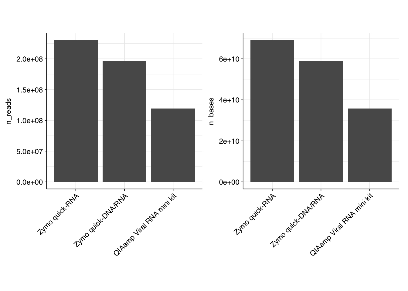
In total, we obtained roughly 550M read pairs, corresponding to roughly 164 Gb of sequencing data. Reads were uniformly 150bp in length. The breakdown of reads was uneven, with the QIAamp kit receiving just over half as many reads – and thus half as many bases – as Zymo quick-RNA.
Data quality appears good, with all libraries passing per-base and per-sequence quality checks as well as per-base N content checks. Sequence composition checks either pass or raise a warning; none fail. Duplication levels are low, with FASTQC predicting less than 10% duplicated sequences for all libraries. The only real issue with sequence quality is a high prevalence of adapter sequences, which is unsurprising for raw sequencing data.
Preprocessing
To remove adapters and trim low-quality sequences, I ran the raw data through FASTP1:
for p in $(cat prefixes.txt); do echo $p; fastp -i raw/${p}_1.fastq.gz -I raw/${p}_2.fastq.gz -o preproc/${p}_fastp_unmerged_1.fastq.gz -O preproc/${p}_fastp_unmerged_2.fastq.gz --merged_out preproc/${p}_fastp_merged.fastq.gz --failed_out preproc/${p}_fastp_failed.fastq.gz --cut_tail --correction --detect_adapter_for_pe --adapter_fasta adapters.fa --merge --trim_poly_x --thread 16; done
With a single 16-thread process, this took a total of 30 minutes to process all six libraries: 12 minutes for Zymo quick-RNA data, 11 minutes for Zymo quick-DNA/RNA data, and 7 minutes for QIAamp Viral RNA mini kit data. All preprocessed libraries subsequently passed FASTQC’s adapter content checks2.
Code
# Import and process paired dataouter_dir_preproc<-file.path(data_dir, "qc/preproc")qc_archives_preproc_paired<-list.files(outer_dir_preproc, pattern ="unmerged.*zip")qc_data_preproc_paired<-suppressMessages(lapply(qc_archives_preproc_paired, function(p)qc_read(file.path(outer_dir_preproc, p), verbose =FALSE)))qc_tab_preproc_paired<-lapply(qc_data_preproc_paired, function(x)extract_qc_data_paired(x, "_fastp_unmerged_\\d.fastq.gz"))%>%bind_rows# Import and process unpaired dataqc_archives_preproc_unpaired<-list.files(outer_dir_preproc, pattern ="_merged.*zip")qc_data_preproc_unpaired<-suppressMessages(lapply(qc_archives_preproc_unpaired, function(p)qc_read(file.path(outer_dir_preproc, p), verbose =FALSE)))qc_tab_preproc_unpaired<-lapply(qc_data_preproc_unpaired, function(x)extract_qc_data_unpaired(x, "_fastp_merged.fastq.gz"))%>%bind_rows# Combineqc_tab_preproc<-bind_rows(qc_tab_preproc_paired, qc_tab_preproc_unpaired)%>%left_join(sample_metadata, by ="sequencing_id")%>%select(sample_id, library_id, kit, sequencing_replicate, read_pair,everything())%>%mutate(stage ="preprocessed")%>%arrange(sample_id, sequencing_replicate, read_pair)qc_tab_preproc
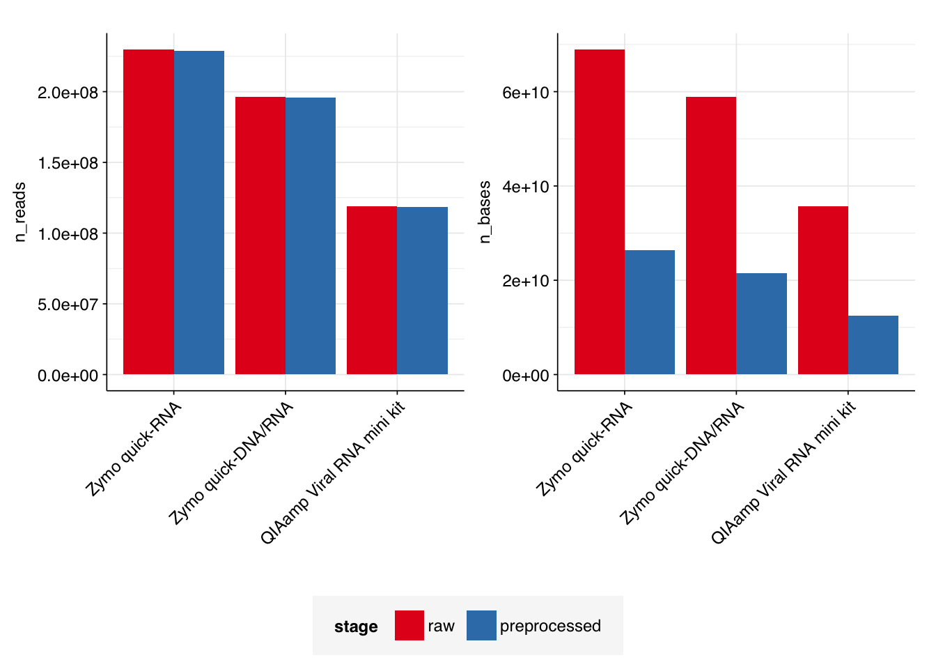
In total, roughly 103 Gb of sequence data (63.1%) was lost during preprocessing. Per-kit losses ranged from 61.7% to 65.1%. Conversely, very few reads (<1%) were discarded entirely.
I was sufficiently surprised by the magnitude of these losses that I checked the number of reads and bases in several files manually to confirm the FASTQC estimates were accurate – they are.
My current best explanation for the scale of the losses is that the fragments being sequenced are primarily small, such that a large number of bases are lost during collapsing of overlapping read pairs. This is consistent with the small fragment sizes that predominate in our Fragment Analyzer data, and the fact that much less material is lost when FASTP is run without collapsing overlapping read pairs (data not shown).
An upside of the large decrease in sequence information caused by collapsing redundant sequence across read pairs is that downstream steps should run substantially faster as a result.
Ribodetection
As DNA sequencing reads, I expected these data to be low in ribosomal sequences. To test this, I ran the data through bbduk, using the same reference sequences described here:
for p in $(cat prefixes.txt); do echo $p;
bbduk.sh in=preproc/${p}_fastp_unmerged_1.fastq.gz in2=preproc/${p}_fastp_unmerged_2.fastq.gz ref=../../riboseqs/SILVA_138.1_LSURef_NR99_tax_silva.fasta.gz,../../riboseqs/SILVA_138.1_SSURef_NR99_tax_silva.fasta.gz out=ribo/${p}_bbduk_unmerged_passed_1.fastq.gz out2=ribo/${p}_bbduk_unmerged_passed_2.fastq.gz outm=ribo/${p}_bbduk_unmerged_failed_1.fastq.gz outm2=ribo/${p}_bbduk_unmerged_failed_2.fastq.gz stats=ribo/${p}_bbduk_unmerged_stats.txt k=30 t=30;
bbduk.sh in=preproc/${p}_fastp_merged.fastq.gz ref=../../riboseqs/SILVA_138.1_LSURef_NR99_tax_silva.fasta.gz,../../riboseqs/SILVA_138.1_SSURef_NR99_tax_silva.fasta.gz out=ribo/${p}_bbduk_merged_passed.fastq.gz outm=ribo/${p}_bbduk_merged_failed.fastq.gz stats=ribo/${p}_bbduk_merged_stats.txt k=30 t=30;
done
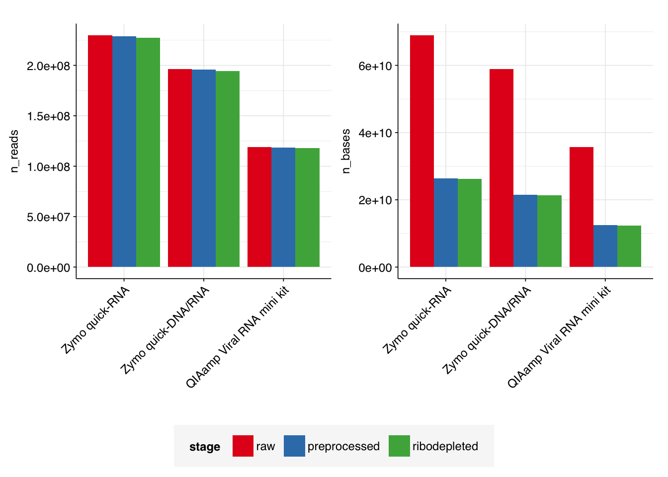
In total, running ribodetection on all six libraries in series took 20 minutes: 8 minutes for Zymo quick-RNA data, 7 minutes for Zymo quick-DNA/RNA data, and 5 minutes for QIAamp Viral RNA mini kit data. As expected, the number of ribosomal reads detected was very low: in total, only 3.6M read pairs (0.67%) were removed during ribodetection, with levels for individual input samples ranging from 0.60% to 0.72%.
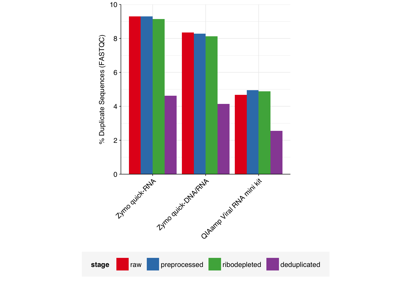
Based on the initial FASTQC results, I expected duplication levels in the ribodepleted data to be low. To confirm this, I performed deduplication with Clumpify as described here3:
for p in $(cat prefixes.txt); do echo $p;
clumpify.sh in=ribo/${p}_bbduk_unmerged_passed_1.fastq.gz in2=ribo/${p}_bbduk_unmerged_passed_2.fastq.gz out=dedup/${p}_clumpify_unmerged_1.fastq.gz out2=dedup/${p}_clumpify_unmerged_2.fastq.gz reorder dedupe t=30;
clumpify.sh in=ribo/${p}_bbduk_merged_passed.fastq.gz out=dedup/${p}_clumpify_merged.fastq.gz reorder dedupe t=30;
done
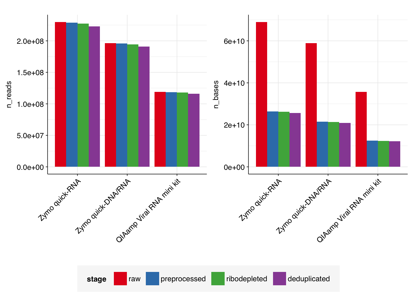
In total, running deduplication on all six libraries in series took 22 minutes: 10 minutes for Zymo quick-RNA data, 8 minutes for Zymo quick-DNA/RNA data, and 4 minutes for QIAamp Viral RNA mini kit data.
As expected, the number of duplicate reads was low: in total, 9.6M read pairs (1.8%) were removed during deduplication, with levels for individual input samples ranging from 1.4% to 2.1%. After deduplication using these parameters, the detected fraction of duplicates identified by FASTQC roughly halved for all samples:
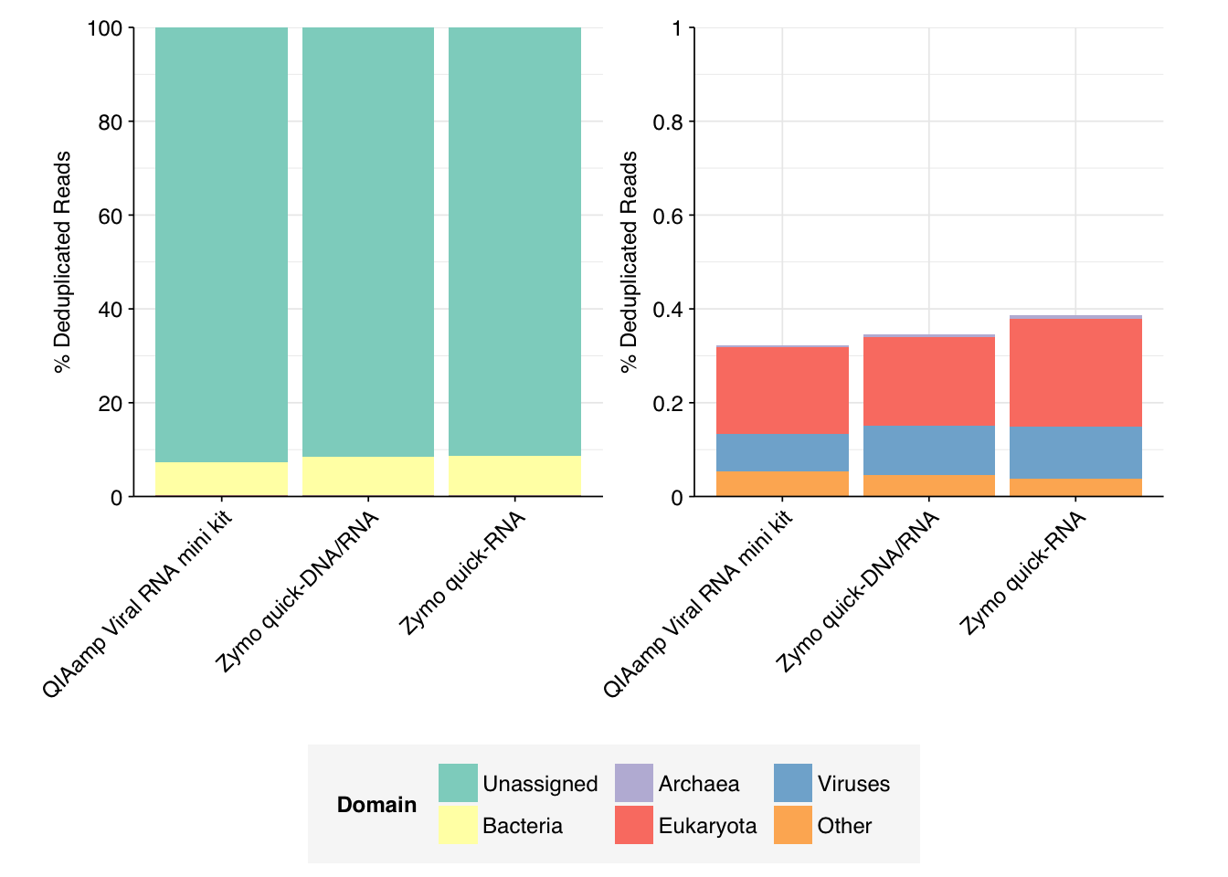
Following deduplication, I ran the data through Kraken2 for taxonomic assignments, using the 16GB Standard database4:
for p in $(cat prefixes.txt); do echo $p;
kraken2 --db ~/kraken-db/ --use-names --paired --threads 30 --output kraken/${p}_unmerged.output --report kraken/${p}_unmerged.report dedup/${p}_clumpify_unmerged_[12].fastq.gz;
kraken2 --db ~/kraken-db/ --use-names --threads 30 --output kraken/${p}_merged.output --report kraken/${p}_merged.report dedup/${p}_clumpify_merged.fastq.gz; cat kraken/${p}_unmerged.output kraken/${p}_merged.output > kraken/${p}.output;
done
In all cases, most of the reads (>91%) were unassigned, and most of the rest (>7%) were bacterial. Assigned archaea, eukaryote, and virus reads all made up a very small fraction of the data for all samples.
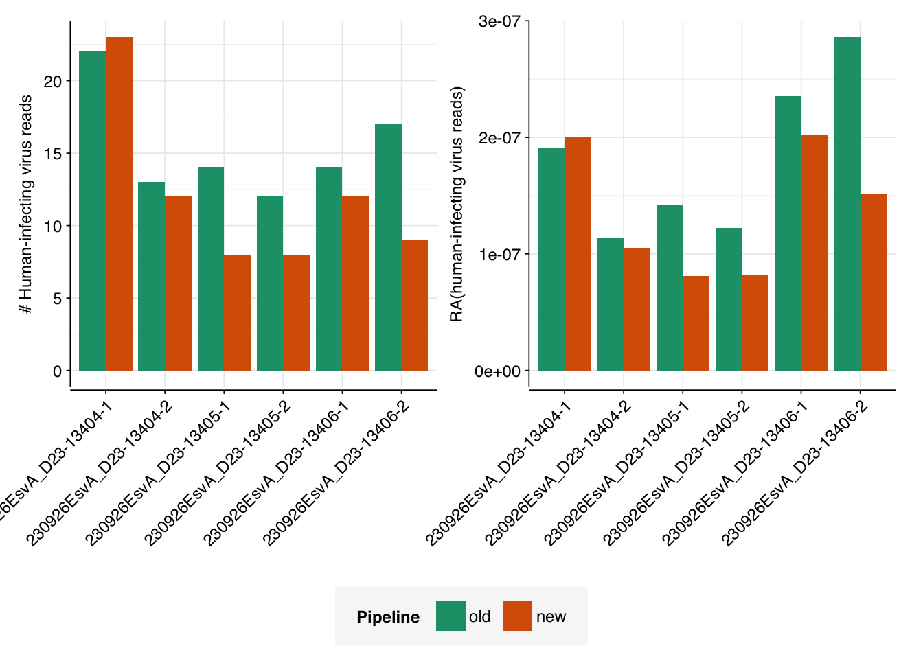
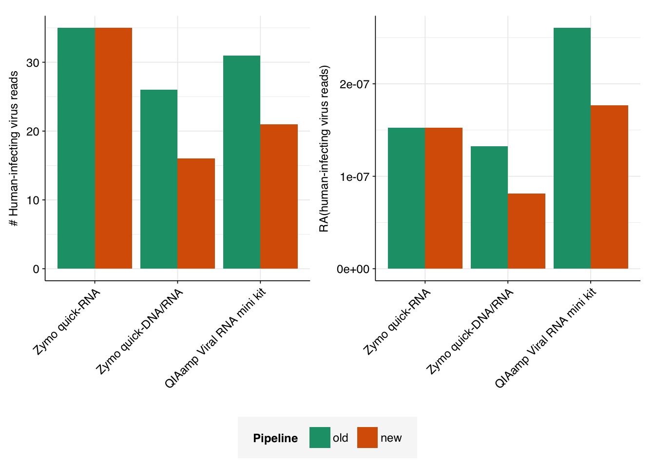
Finally, I calculated the number of reads assigned to human-infecting viruses, using scripts based on the cladecounts and allmatches functions from the public pipeline. The number of resulting read assignments varied from just over half as many as in the private dashboard, to slightly more than that number:
I’m not sure what exactly is giving rise to the discrepancy between the two pipelines. While some degree of disagreement between two different pipelines isn’t surprising, it would be good to have a deeper understanding of what’s causing it, and which pipeline is giving results that are more “believable”. I’ll look more deeply into this in a subsequent notebook entry.
Footnotes
I initially ran FASTP without collapsing read pairs (--merge), as this makes for easier and more elegant downstream processing. However, this led to erroneous overidentification of read taxa during the Kraken2 analysis step by spuriously duplicating overlapping sequences. As such, I grudgingly implemented read-pair collapsing here as in the original pipeline.↩︎
I initially ran FASTP without using pre-specified adapter sequences (–adapter_fasta adapters.fa). In most cases, FASTP successfully auto-detected and removed adapters, resulting in very low adapter prevalence in the preprocessed files. However, adapter trimming failed for two files: 230926EsvA_D23-13406-1_fastp_2.fastq.gz and 230926EsvA_D23-13406-2_fastp_2.fastq.gz. Digging into the FASTP logs, it looks like it failed to identify an adapter sequence for these files, resulting in inadequate adapter trimming. Rerunning FASTP while explicitly passing the Illumina TruSeq adapter sequences (alongside automated adapter detection) solved this problem in this instance.↩︎
After running this, I realized this is probably an underestimate of the level of duplication, as it’s not counting duplicate reads from the same library sequenced on different lanes. I’ll look into cross-lane duplicates as part of a deeper investigation of duplication levels that I plan to do a bit later.↩︎
In the future, I plan to look at the effect of using different Kraken2 databases on read assignment, but for now I’m sticking with the database used in the main pipeline.↩︎
Source Code
---title: "Initial analysis of Project Runway protocol testing data"subtitle: ""author: "Will Bradshaw"date: 2023-10-31format: html: code-fold: true code-tools: true code-link: true df-print: pagededitor: visualtitle-block-banner: black---```{r}#| label: load-packages#| include: falselibrary(tidyverse)library(cowplot)library(patchwork)library(fastqcr)source("../scripts/aux_plot-theme.R")```On 2023-10-23, we received the first batch of sequencing data from our wastewater protocol optimization work. This notebook contains the output of initial QC and analysis for this data.# BackgroundWe carried out concentration and extraction on primary sludge samples from wastewater treatment plant A (WTP-A) using three different nucleic-acid extraction kits:- Zymo quick-RNA kit- Zymo quick-DNA/RNA kit- QIAamp Viral RNA mini kitWe [previously](https://data.securebio.org/wills-public-notebook/notebooks/2023-09-12_settled-solids-extraction-test.html) looked at total NA yield, qPCR and Fragment Analyzer results for these extractions as well as several other kits. We selected these three kits as the most promising, and sent them for sequencing to further characterize the quality of the extractions. Two replicate extractions per kit were sent for sequencing; one (replicate A) underwent RNA sequencing only while the other (replicate C) underwent both DNA and RNA sequencing. We also sent two samples extracted in a previous experiment (using the QIAamp kit) for RNA sequencing.So far, only the DNA sequencing data is available, corresponding to one replicate per kit, or three samples total.# The raw dataThe raw data from the BMC consists of sixteen FASTQ files, corresponding to paired-end data from eight sequencing libraries. This is rather more than the three libraries we were expecting; digging into this, each submitted sample seems to have been sequenced twice, and we also have two pairs of FASTQ files corresponding to "unmapped barcodes" (`231016_78783_6418E_L1_{1,2}_sequence_unmapped_barcodes.fastq` and `231016_78783_6418E_L2_{1,2}_sequence_unmapped_barcodes.fastq`).Given that these have the same sequencing date and other annotations, and that (according to communication from the BMC) each submitted library has the same index barcode in both cases, my guess is that each sample was sequenced on both lanes of the AVITI flow cell. However, it would be useful to check with BMC and confirm this.The data from the BMC helpfully comes with FASTQC files attached, which we can use to look at the quality of the raw data.```{r}data_dir <-"../data/2023-10-24_pr-dna"outer_dir <-file.path(data_dir, "qc/raw")qc_archives <-list.files(outer_dir, pattern ="*.zip")qc_data <-suppressMessages(lapply(qc_archives, function(p) qc_read(file.path(outer_dir, p), verbose =FALSE)))# Sample mappingsample_metadata <-read_csv("../data/2023-10-24_pr-dna/sample-metadata.csv", show_col_types =FALSE)# Compute approximate number of sequence bases from sequence length distribution tablecompute_n_bases <-function(sld){ min_lengths <-sub("-.*", "", sld$Length) %>% as.numeric max_lengths <-sub(".*-", "", sld$Length) %>% as.numeric mean_lengths <- (min_lengths + max_lengths)/2 sld2 <-mutate(sld, Length_mean = mean_lengths) n_bases <-sum(sld2$Count * sld2$Length_mean)return(n_bases)}# FASTQC processing functionsextract_qc_data_base <-function(qc){ filename <-filter(qc$basic_statistics, Measure =="Filename")$Value n_reads <-filter(qc$basic_statistics, Measure =="Total Sequences")$Value %>% as.integer n_bases <-compute_n_bases(qc$sequence_length_distribution) pc_dup <-100-qc$total_deduplicated_percentage per_base_quality <-filter(qc$summary, module =="Per base sequence quality")$status per_sequence_quality <-filter(qc$summary, module =="Per sequence quality scores")$status per_base_composition <-filter(qc$summary, module =="Per base sequence content")$status per_sequence_composition <-filter(qc$summary, module =="Per sequence GC content")$status per_base_n_content <-filter(qc$summary, module =="Per base N content")$status adapter_content <-filter(qc$summary, module =="Adapter Content")$status tab_out <-tibble(n_reads = n_reads,n_bases = n_bases,pc_dup = pc_dup,per_base_quality = per_base_quality,per_sequence_quality = per_sequence_quality,per_base_composition = per_base_composition,per_sequence_composition = per_sequence_composition,per_base_n_content = per_base_n_content,adapter_content = adapter_content,filename = filename)return(tab_out)}extract_qc_data_paired <-function(qc, id_pattern, pair_pattern =".*_(\\d)[_.].*"){ base <-extract_qc_data_base(qc) filename <- base$filename[1] prefix <-sub(id_pattern, "", filename) read_pair <-sub(pair_pattern, "\\1", filename) tab_out <- base %>%mutate(sequencing_id = prefix, read_pair = read_pair) %>%select(sequencing_id, read_pair, everything())return(tab_out)}extract_qc_data_unpaired <-function(qc, id_pattern){ base <-extract_qc_data_base(qc) filename <- base$filename[1] prefix <-sub(id_pattern, "", filename) tab_out <- base %>%mutate(sequencing_id = prefix) %>%select(sequencing_id, everything())return(tab_out)}# Generate and show sample tablepattern_raw <-"_\\d_sequence.fastq.*$"qc_tab <-lapply(qc_data, function(x) extract_qc_data_paired(x, pattern_raw)) %>% bind_rows %>%inner_join(sample_metadata, by ="sequencing_id") %>%select(sample_id, library_id, kit, sequencing_replicate, read_pair, everything()) %>%mutate(stage ="raw")rm(qc_data) qc_tab```In total, we obtained roughly 550M read pairs, corresponding to roughly 164 Gb of sequencing data. Reads were uniformly 150bp in length. The breakdown of reads was uneven, with the QIAamp kit receiving just over half as many reads -- and thus half as many bases -- as Zymo quick-RNA.```{r}n_reads_1 <- qc_tab %>%group_by(sample_id, kit, read_pair) %>%summarize(n_reads =sum(as.integer(n_reads)), n_bases =sum(n_bases), .groups ="drop") %>%mutate(kit =fct_inorder(kit))n_bases_1 <- n_reads_1 %>%group_by(sample_id, kit) %>%summarize(n_bases =sum(n_bases), .groups ="drop")theme_kit <- theme_base +theme(aspect.ratio =1,axis.text.x =element_text(hjust =1, angle =45),axis.title.x =element_blank())g_reads_raw <-ggplot(n_reads_1 %>%filter(read_pair ==1), aes(x=kit, y=n_reads)) +geom_col() + theme_kitg_bases_raw <-ggplot(n_bases_1, aes(x=kit, y=n_bases)) +geom_col() + theme_base + theme_kitg_reads_raw + g_bases_raw```Data quality appears good, with all libraries passing per-base and per-sequence quality checks as well as per-base N content checks. Sequence composition checks either pass or raise a warning; none fail. Duplication levels are low, with FASTQC predicting less than 10% duplicated sequences for all libraries. The only real issue with sequence quality is a high prevalence of adapter sequences, which is unsurprising for raw sequencing data.# PreprocessingTo remove adapters and trim low-quality sequences, I ran the raw data through FASTP[^1]:[^1]: I initially ran FASTP without collapsing read pairs (`--merge`), as this makes for easier and more elegant downstream processing. However, this led to erroneous overidentification of read taxa during the Kraken2 analysis step by spuriously duplicating overlapping sequences. As such, I grudgingly implemented read-pair collapsing here as in the original pipeline.``` for p in $(cat prefixes.txt); do echo $p; fastp -i raw/${p}_1.fastq.gz -I raw/${p}_2.fastq.gz -o preproc/${p}_fastp_unmerged_1.fastq.gz -O preproc/${p}_fastp_unmerged_2.fastq.gz --merged_out preproc/${p}_fastp_merged.fastq.gz --failed_out preproc/${p}_fastp_failed.fastq.gz --cut_tail --correction --detect_adapter_for_pe --adapter_fasta adapters.fa --merge --trim_poly_x --thread 16; done```With a single 16-thread process, this took a total of 30 minutes to process all six libraries: 12 minutes for Zymo quick-RNA data, 11 minutes for Zymo quick-DNA/RNA data, and 7 minutes for QIAamp Viral RNA mini kit data. All preprocessed libraries subsequently passed FASTQC's adapter content checks[^2].[^2]: I initially ran FASTP without using pre-specified adapter sequences (`–adapter_fasta adapters.fa`). In most cases, FASTP successfully auto-detected and removed adapters, resulting in very low adapter prevalence in the preprocessed files. However, adapter trimming failed for two files: `230926EsvA_D23-13406-1_fastp_2.fastq.gz` and `230926EsvA_D23-13406-2_fastp_2.fastq.gz`. Digging into the FASTP logs, it looks like it failed to identify an adapter sequence for these files, resulting in inadequate adapter trimming. Rerunning FASTP while explicitly passing the Illumina TruSeq adapter sequences (alongside automated adapter detection) solved this problem in this instance.```{r}# Import and process paired dataouter_dir_preproc <-file.path(data_dir, "qc/preproc")qc_archives_preproc_paired <-list.files(outer_dir_preproc, pattern ="unmerged.*zip")qc_data_preproc_paired <-suppressMessages(lapply(qc_archives_preproc_paired, function(p) qc_read(file.path(outer_dir_preproc, p), verbose =FALSE)))qc_tab_preproc_paired <-lapply(qc_data_preproc_paired, function(x)extract_qc_data_paired(x, "_fastp_unmerged_\\d.fastq.gz")) %>% bind_rows# Import and process unpaired dataqc_archives_preproc_unpaired <-list.files(outer_dir_preproc, pattern ="_merged.*zip")qc_data_preproc_unpaired <-suppressMessages(lapply(qc_archives_preproc_unpaired, function(p) qc_read(file.path(outer_dir_preproc, p), verbose =FALSE)))qc_tab_preproc_unpaired <-lapply(qc_data_preproc_unpaired, function(x)extract_qc_data_unpaired(x, "_fastp_merged.fastq.gz")) %>% bind_rows# Combineqc_tab_preproc <-bind_rows(qc_tab_preproc_paired, qc_tab_preproc_unpaired) %>%left_join(sample_metadata, by ="sequencing_id") %>%select(sample_id, library_id, kit, sequencing_replicate, read_pair,everything()) %>%mutate(stage ="preprocessed") %>%arrange(sample_id, sequencing_replicate, read_pair)qc_tab_preproc``````{r}# Calculate per-stage read and base countsqc_tab_2 <-bind_rows(qc_tab, qc_tab_preproc) %>%mutate(stage =fct_inorder(stage), kit =fct_inorder(kit))n_reads_2 <- qc_tab_2 %>%group_by(sample_id, kit, read_pair, stage) %>%summarize(n_reads =sum(as.integer(n_reads)),n_bases =sum(n_bases), .groups ="drop")n_bases_2 <- n_reads_2 %>%group_by(sample_id, kit, stage) %>%summarize(n_bases =sum(n_bases), .groups ="drop")n_reads_2_out <- n_reads_2 %>%filter(read_pair ==1|is.na(read_pair)) %>%group_by(sample_id, kit, stage) %>%summarize(n_reads =sum(n_reads), .groups ="drop")# Plotg_reads_preproc <- n_reads_2_out %>%ggplot(aes(x=kit, y=n_reads, fill=stage)) +geom_col(position ="dodge") +scale_fill_brewer(palette ="Set1") + theme_kitg_bases_preproc <- n_bases_2 %>%ggplot(aes(x=kit, y=n_bases, fill=stage)) +geom_col(position ="dodge") +scale_fill_brewer(palette ="Set1") + theme_kit +theme(legend.position ="none")g_preproc_legend <-get_legend(g_reads_preproc)g_reads_preproc_2 <- g_reads_preproc +theme(legend.position ="none")plot_grid(g_reads_preproc_2 + g_bases_preproc, g_preproc_legend, nrow =2, rel_heights =c(1,0.15))```In total, roughly 103 Gb of sequence data (63.1%) was lost during preprocessing. Per-kit losses ranged from 61.7% to 65.1%. Conversely, very few reads (\<1%) were discarded entirely.I was sufficiently surprised by the magnitude of these losses that I checked the number of reads and bases in several files manually to confirm the FASTQC estimates were accurate -- they are.My current best explanation for the scale of the losses is that the fragments being sequenced are primarily small, such that a large number of bases are lost during collapsing of overlapping read pairs. This is consistent with the small fragment sizes that predominate in our Fragment Analyzer data, and the fact that much less material is lost when FASTP is run without collapsing overlapping read pairs (data not shown).An upside of the large decrease in sequence information caused by collapsing redundant sequence across read pairs is that downstream steps should run substantially faster as a result.# RibodetectionAs DNA sequencing reads, I expected these data to be low in ribosomal sequences. To test this, I ran the data through bbduk, using the same reference sequences described [here](https://data.securebio.org/wills-public-notebook/notebooks/2023-10-13_rrna-removal.html):``` for p in $(cat prefixes.txt); do echo $p; bbduk.sh in=preproc/${p}_fastp_unmerged_1.fastq.gz in2=preproc/${p}_fastp_unmerged_2.fastq.gz ref=../../riboseqs/SILVA_138.1_LSURef_NR99_tax_silva.fasta.gz,../../riboseqs/SILVA_138.1_SSURef_NR99_tax_silva.fasta.gz out=ribo/${p}_bbduk_unmerged_passed_1.fastq.gz out2=ribo/${p}_bbduk_unmerged_passed_2.fastq.gz outm=ribo/${p}_bbduk_unmerged_failed_1.fastq.gz outm2=ribo/${p}_bbduk_unmerged_failed_2.fastq.gz stats=ribo/${p}_bbduk_unmerged_stats.txt k=30 t=30;bbduk.sh in=preproc/${p}_fastp_merged.fastq.gz ref=../../riboseqs/SILVA_138.1_LSURef_NR99_tax_silva.fasta.gz,../../riboseqs/SILVA_138.1_SSURef_NR99_tax_silva.fasta.gz out=ribo/${p}_bbduk_merged_passed.fastq.gz outm=ribo/${p}_bbduk_merged_failed.fastq.gz stats=ribo/${p}_bbduk_merged_stats.txt k=30 t=30; done```In total, running ribodetection on all six libraries in series took 20 minutes: 8 minutes for Zymo quick-RNA data, 7 minutes for Zymo quick-DNA/RNA data, and 5 minutes for QIAamp Viral RNA mini kit data. As expected, the number of ribosomal reads detected was very low: in total, only 3.6M read pairs (0.67%) were removed during ribodetection, with levels for individual input samples ranging from 0.60% to 0.72%.```{r}# Import and process paired dataouter_dir_ribo <-file.path(data_dir, "qc/ribo")qc_archives_ribo_paired <-list.files(outer_dir_ribo, pattern ="unmerged_passed.*zip")qc_data_ribo_paired <-suppressMessages(lapply(qc_archives_ribo_paired, function(p) qc_read(file.path(outer_dir_ribo, p), verbose =FALSE)))qc_tab_ribo_paired <-lapply(qc_data_ribo_paired, function(x)extract_qc_data_paired(x, "_bbduk_unmerged_passed_\\d.fastq.gz")) %>% bind_rows# Import and process unpaired dataqc_archives_ribo_unpaired <-list.files(outer_dir_ribo, pattern ="_merged_passed.*zip")qc_data_ribo_unpaired <-suppressMessages(lapply(qc_archives_ribo_unpaired, function(p) qc_read(file.path(outer_dir_ribo, p), verbose =FALSE)))qc_tab_ribo_unpaired <-lapply(qc_data_ribo_unpaired, function(x)extract_qc_data_unpaired(x, "_bbduk_merged_passed.fastq.gz")) %>% bind_rows# Combineqc_tab_ribo <-bind_rows(qc_tab_ribo_paired, qc_tab_ribo_unpaired) %>%left_join(sample_metadata, by ="sequencing_id") %>%select(sample_id, library_id, kit, sequencing_replicate, read_pair,everything()) %>%mutate(stage ="ribodepleted") %>%arrange(sample_id, sequencing_replicate, read_pair)# Calculate per-stage read and base countsqc_tab_3 <-bind_rows(qc_tab, qc_tab_preproc, qc_tab_ribo) %>%mutate(stage =fct_inorder(stage), kit =fct_inorder(kit))n_reads_3 <- qc_tab_3 %>%group_by(sample_id, kit, read_pair, stage) %>%summarize(n_reads =sum(as.integer(n_reads)),n_bases =sum(n_bases), .groups ="drop")n_bases_3 <- n_reads_3 %>%group_by(sample_id, kit, stage) %>%summarize(n_bases =sum(n_bases), .groups ="drop")n_reads_3_out <- n_reads_3 %>%filter(read_pair ==1|is.na(read_pair)) %>%group_by(sample_id, kit, stage) %>%summarize(n_reads =sum(n_reads), .groups ="drop")# Plotg_reads_ribo <- n_reads_3_out %>%ggplot(aes(x=kit, y=n_reads, fill=stage)) +geom_col(position ="dodge") +scale_fill_brewer(palette ="Set1") + theme_kitg_bases_ribo <- n_bases_3 %>%ggplot(aes(x=kit, y=n_bases, fill=stage)) +geom_col(position ="dodge") +scale_fill_brewer(palette ="Set1") + theme_kit +theme(legend.position ="none")g_ribo_legend <-get_legend(g_reads_ribo)g_reads_ribo_2 <- g_reads_ribo +theme(legend.position ="none")plot_grid(g_reads_ribo_2 + g_bases_ribo, g_ribo_legend, nrow =2, rel_heights =c(1,0.15))```# DeduplicationBased on the initial FASTQC results, I expected duplication levels in the ribodepleted data to be low. To confirm this, I performed deduplication with Clumpify as described [here](https://data.securebio.org/wills-public-notebook/notebooks/2023-10-19_deduplication.html)[^3]:[^3]: After running this, I realized this is probably an underestimate of the level of duplication, as it's not counting duplicate reads from the same library sequenced on different lanes. I'll look into cross-lane duplicates as part of a deeper investigation of duplication levels that I plan to do a bit later.``` for p in $(cat prefixes.txt); do echo $p; clumpify.sh in=ribo/${p}_bbduk_unmerged_passed_1.fastq.gz in2=ribo/${p}_bbduk_unmerged_passed_2.fastq.gz out=dedup/${p}_clumpify_unmerged_1.fastq.gz out2=dedup/${p}_clumpify_unmerged_2.fastq.gz reorder dedupe t=30; clumpify.sh in=ribo/${p}_bbduk_merged_passed.fastq.gz out=dedup/${p}_clumpify_merged.fastq.gz reorder dedupe t=30; done```In total, running deduplication on all six libraries in series took 22 minutes: 10 minutes for Zymo quick-RNA data, 8 minutes for Zymo quick-DNA/RNA data, and 4 minutes for QIAamp Viral RNA mini kit data.```{r}# Import and process paired dataouter_dir_dedup <-file.path(data_dir, "qc/dedup")qc_archives_dedup_paired <-list.files(outer_dir_dedup, pattern ="unmerged.*zip")qc_data_dedup_paired <-suppressMessages(lapply(qc_archives_dedup_paired, function(p) qc_read(file.path(outer_dir_dedup, p), verbose =FALSE)))qc_tab_dedup_paired <-lapply(qc_data_dedup_paired, function(x)extract_qc_data_paired(x, "_clumpify_unmerged_\\d.fastq.gz")) %>% bind_rows# Import and process unpaired dataqc_archives_dedup_unpaired <-list.files(outer_dir_dedup, pattern ="_merged.*zip")qc_data_dedup_unpaired <-suppressMessages(lapply(qc_archives_dedup_unpaired, function(p) qc_read(file.path(outer_dir_dedup, p), verbose =FALSE)))qc_tab_dedup_unpaired <-lapply(qc_data_dedup_unpaired, function(x)extract_qc_data_unpaired(x, "_clumpify_merged.fastq.gz")) %>% bind_rows# Combineqc_tab_dedup <-bind_rows(qc_tab_dedup_paired, qc_tab_dedup_unpaired) %>%left_join(sample_metadata, by ="sequencing_id") %>%select(sample_id, library_id, kit, sequencing_replicate, read_pair,everything()) %>%mutate(stage ="deduplicated") %>%arrange(sample_id, sequencing_replicate, read_pair)# Calculate per-stage read and base countsqc_tab_4 <-bind_rows(qc_tab, qc_tab_preproc, qc_tab_ribo, qc_tab_dedup) %>%mutate(stage =fct_inorder(stage), kit =fct_inorder(kit))n_reads_4 <- qc_tab_4 %>%group_by(sample_id, kit, read_pair, stage) %>%summarize(n_reads =sum(as.integer(n_reads)),n_bases =sum(n_bases), .groups ="drop")n_bases_4 <- n_reads_4 %>%group_by(sample_id, kit, stage) %>%summarize(n_bases =sum(n_bases), .groups ="drop")n_reads_4_out <- n_reads_4 %>%filter(read_pair ==1|is.na(read_pair)) %>%group_by(sample_id, kit, stage) %>%summarize(n_reads =sum(n_reads), .groups ="drop")# Plotg_reads_dedup <- n_reads_4_out %>%ggplot(aes(x=kit, y=n_reads, fill=stage)) +geom_col(position ="dodge") +scale_fill_brewer(palette ="Set1") + theme_kitg_bases_dedup <- n_bases_4 %>%ggplot(aes(x=kit, y=n_bases, fill=stage)) +geom_col(position ="dodge") +scale_fill_brewer(palette ="Set1") + theme_kit +theme(legend.position ="none")g_dedup_legend <-get_legend(g_reads_dedup)g_reads_dedup_2 <- g_reads_dedup +theme(legend.position ="none")plot_grid(g_reads_dedup_2 + g_bases_dedup, g_dedup_legend, nrow =2, rel_heights =c(1,0.15))```As expected, the number of duplicate reads was low: in total, 9.6M read pairs (1.8%) were removed during deduplication, with levels for individual input samples ranging from 1.4% to 2.1%. After deduplication using these parameters, the detected fraction of duplicates identified by FASTQC roughly halved for all samples:```{r}n_dups <- qc_tab_4 %>%group_by(sample_id, kit, stage) %>%mutate(n_reads =as.integer(n_reads)) %>%summarize(pc_dup =sum(n_reads * pc_dup/100)/sum(n_reads)*100, .groups ="drop")g_dups <- n_dups %>%ggplot(aes(x=kit, y=pc_dup, fill=stage)) +geom_col(position ="dodge") +scale_fill_brewer(palette ="Set1") +scale_y_continuous(name ="% Duplicate Sequences (FASTQC)", expand =c(0,0),limits =c(0,10), breaks =seq(0,100,2)) + theme_base +theme(aspect.ratio =1, axis.title.x =element_blank(),axis.text.x =element_text(hjust =1, angle =45))g_dups```# Kraken2 -- Initial AssignmentsFollowing deduplication, I ran the data through Kraken2 for taxonomic assignments, using the 16GB Standard database[^4]:[^4]: In the future, I plan to look at the effect of using different Kraken2 databases on read assignment, but for now I'm sticking with the database used in the main pipeline.``` for p in $(cat prefixes.txt); do echo $p; kraken2 --db ~/kraken-db/ --use-names --paired --threads 30 --output kraken/${p}_unmerged.output --report kraken/${p}_unmerged.report dedup/${p}_clumpify_unmerged_[12].fastq.gz; kraken2 --db ~/kraken-db/ --use-names --threads 30 --output kraken/${p}_merged.output --report kraken/${p}_merged.report dedup/${p}_clumpify_merged.fastq.gz; cat kraken/${p}_unmerged.output kraken/${p}_merged.output > kraken/${p}.output; done```In all cases, most of the reads (\>91%) were unassigned, and most of the rest (\>7%) were bacterial. Assigned archaea, eukaryote, and virus reads all made up a very small fraction of the data for all samples.```{r}kraken_domains_path <-file.path(data_dir, "kraken-domains.csv")kraken_domains <-read_csv(kraken_domains_path, show_col_types =FALSE) %>%left_join(sample_metadata, by =c("library_id", "sequencing_id", "sequencing_replicate")) %>%select(sample_id, library_id, kit, sequencing_replicate, everything())kraken_domains_gathered <- kraken_domains %>%select(-n_total) %>%gather(domain, n_reads, -sample_id, -library_id, -kit, -sequencing_replicate, -sequencing_id, -index) %>%mutate(domain =str_to_sentence(sub("n_", "", domain)),domain =fct_inorder(domain)) %>%group_by(sample_id, kit, domain) %>%summarize(n_reads =sum(n_reads), .groups ="drop_last") %>%mutate(p_reads = n_reads/sum(n_reads))g_domains <- kraken_domains_gathered %>%ggplot(aes(x=kit, y=p_reads, fill = domain)) +geom_col(position ="stack") +scale_fill_brewer(palette ="Set3", name ="Domain") +scale_y_continuous(name ="% Deduplicated Reads", expand =c(0,0),limits =c(0,1), breaks =seq(0,1,0.2),labels =function(y) y *100) + theme_kitg_domains_minor <- kraken_domains_gathered %>%filter(! domain %in%c("Unassigned", "Bacteria")) %>%ggplot(aes(x=kit, y=p_reads, fill = domain)) +geom_col(position ="stack") +scale_fill_manual(values = scales::brewer_pal(palette ="Set3")(8)[-c(1,2)],name ="Domain") +scale_y_continuous(name ="% Deduplicated Reads", expand =c(0,0),limits =c(0,0.01), breaks =seq(0,0.01,0.002),labels =function(y) y *100) + theme_kit +theme(legend.position ="none")g_domains_legend <-get_legend(g_domains)g_domains_2 <- g_domains +theme(legend.position ="none")plot_grid(g_domains_2 + g_domains_minor, g_domains_legend, nrow =2, rel_heights =c(1,0.2))```# Kraken2 -- Human-Infecting VirusesFinally, I calculated the number of reads assigned to human-infecting viruses, using scripts based on the `cladecounts` and `allmatches` functions from [the public pipeline](https://github.com/naobservatory/mgs-pipeline/blob/main/run.py). The number of resulting read assignments varied from just over half as many as in the private dashboard, to slightly more than that number:```{r}hv_counts_path <-file.path(data_dir, "hv-counts.csv")hv_counts <-read_csv(hv_counts_path, show_col_types =FALSE) %>%left_join(sample_metadata, by =c("library_id", "sequencing_id", "sequencing_replicate")) %>%select(sample_id, library_id, kit, sequencing_replicate, everything())hv_counts_gathered <- hv_counts %>%select(-index) %>%gather(pipeline, n_hv, -sample_id, -library_id, -kit, -sequencing_replicate, -sequencing_id, -n_total) %>%mutate(pipeline =sub("hv_", "", pipeline),pipeline =fct_inorder(pipeline),p_hv = n_hv/n_total)g_hv_n <-ggplot(hv_counts_gathered, aes(x=sequencing_id, y=n_hv, fill=pipeline)) +geom_col(position ="dodge") +scale_y_continuous(name ="# Human-infecting virus reads") +scale_fill_brewer(palette ="Dark2", name ="Pipeline") + theme_kitg_hv_p <-ggplot(hv_counts_gathered, aes(x=sequencing_id, y=p_hv, fill=pipeline)) +geom_col(position ="dodge") +scale_y_continuous(name ="RA(human-infecting virus reads)") +scale_fill_brewer(palette ="Dark2", name ="Pipeline") + theme_kit +theme(legend.position ="none")g_hv_legend <-get_legend(g_hv_n)g_hv_n_2 <- g_hv_n +theme(legend.position ="none")plot_grid(g_hv_n_2 + g_hv_p, g_hv_legend, nrow =2, rel_heights =c(1,0.15))```Summarizing over kits, the results are as follows:```{r}hv_counts_summ <- hv_counts_gathered %>%mutate(kit =fct_inorder(kit)) %>%group_by(sample_id, kit, pipeline) %>%summarize(n_total =sum(n_total), n_hv =sum(n_hv), .groups ="drop") %>%mutate(p_hv = n_hv/n_total)g_hv_summ_n <-ggplot(hv_counts_summ, aes(x=kit, y=n_hv, fill=pipeline)) +geom_col(position ="dodge") +scale_y_continuous(name ="# Human-infecting virus reads") +scale_fill_brewer(palette ="Dark2", name ="Pipeline") + theme_kitg_hv_summ_p <-ggplot(hv_counts_summ, aes(x=kit, y=p_hv, fill=pipeline)) +geom_col(position ="dodge") +scale_y_continuous(name ="RA(human-infecting virus reads)") +scale_fill_brewer(palette ="Dark2", name ="Pipeline") + theme_kit +theme(legend.position ="none")g_hv_summ_legend <-get_legend(g_hv_summ_n)g_hv_summ_n_2 <- g_hv_summ_n +theme(legend.position ="none")plot_grid(g_hv_summ_n_2 + g_hv_summ_p, g_hv_summ_legend, nrow =2, rel_heights =c(1,0.15))```I'm not sure what exactly is giving rise to the discrepancy between the two pipelines. While some degree of disagreement between two different pipelines isn't surprising, it would be good to have a deeper understanding of what's causing it, and which pipeline is giving results that are more "believable". I'll look more deeply into this in a subsequent notebook entry.