NAO Cost Estimate MVP – Optimizing the sampling interval
Author
Dan Rice
Published
February 13, 2024
Modified
March 31, 2024
Background
See previous notebook. The goal of this notebook is to use our simple, deterministic cost estimate to answer the question:
How often should we process and sequence samples?
We want to understand the tradeoff between:
catching the virus earlier by sampling more frequently, and
saving on processing costs by sampling less frequently.
To this end, we posit a two-component cost model:
Per-read sequencing costs, and
Per-sample processing costs
and find the optimal sampling interval \(\delta t\) that minimizes total costs, while sequencing to sufficient depth per sample \(n\) to detect a virus by cumulative incidence \(\hat{c}\).
A two-component cost model
Consider the cost averaged over a long time interval \(T\) in which we will take many samples. If we collect and process samples every \(\delta t\) days, we will take \(T / \delta t\) samples in this interval. If we sample \(n\) reads per sample, our total sequencing depth is \(n \frac{\delta t}{T}\) reads. Assume that our costs can be divided into a per-sample cost \(d_s\) (including costs of collection, transportation, and processing for sequencing) and a per-read cost \(d_r\) of sequencing. (Note: the \(d\) is sort of awkward because we’ve already used \(c\) for “cumulative incidence”. You can think of it as standing for “dollars”.)
We will seek to minimize the total cost of detection: \[
d_{\text{tot}} = d_s \frac{T}{\delta t} + d_r \frac{nT}{\delta t}.
\] Equivalently, we can divide by the arbitrary time-interval \(T\) to get the total rate of spending: \[
\frac{d_{\text{tot}}}{T} = \frac{d_s}{\delta t} + d_r \frac{n}{\delta t}.
\]
In our previous post, we found that the read depth per time required to detect a virus by the time it reaches cumulative incidence \(\hat{c}\) is:
where the function \(f\) depends on the sampling scheme. Substituting this into the rate of spending, we have: \[
\frac{d_{\text{tot}}}{T} = \frac{d_s}{\delta t} + (r + \beta) \left(\frac{\hat{K}}{b \hat{c}}\right) e^{r t_d} d_r f(r \delta t).
\]
In the next section, we will find the value of \(\delta t\) that minimizes the rate of spending.
Limitations of the two-component model
We assume that we process each sample as it comes in. In practice, we could stockpile a set of \(m\) samples and process them simultaneously. This would require splitting out the cost of sampling from the cost of sample prep.
We do not consider the fact that sequencing (and presumably to some extent sample prep) unit costs decrease with greater depth. (I.e., it’s cheaper per-read to do bigger runs.)
We neglect the “batch” effects of sequencing. Typically you buy sequencing in units of “lanes” rather than asking for an arbitrary number of reads. This will introduce threshold effects, where we want to batach our samples to use lanes efficiently.
We do not account for fixed costs that accumulate per unit time regardless of our sampling and sequencing protocols. These do not affect the optimization here, but they do add to the total cost of the system.
Optimizing the sampling interval
To find the optimal \(\delta t\), we look for a zero of the derivative of spending rate:
To get any farther, we need to specify \(f\) and therefore a sampling scheme. [Note: If we give some general properties of \(f\), we can say some things here that are general to the sampling scheme]
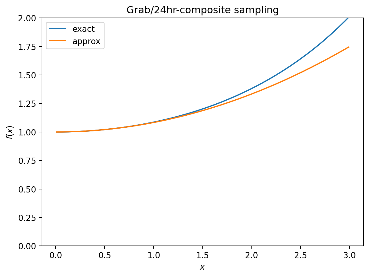
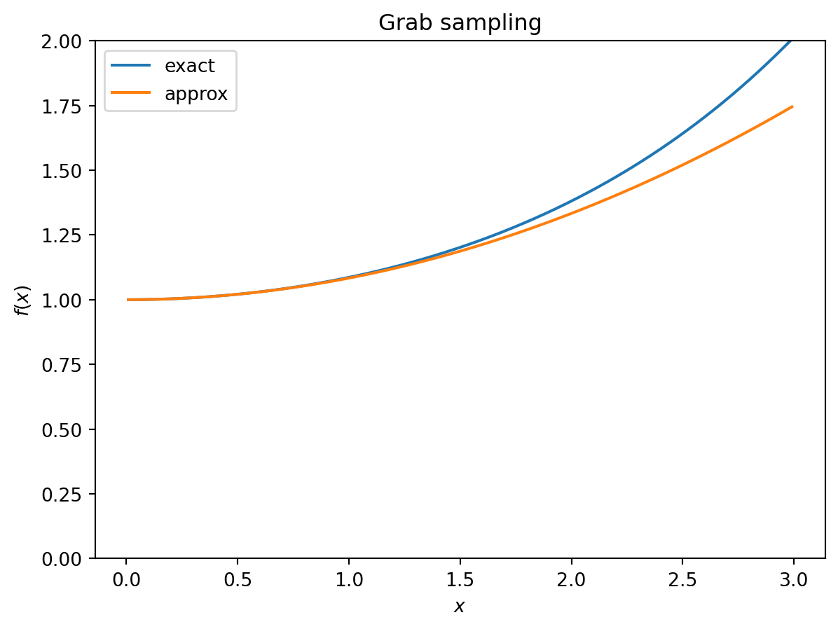
Grab sampling
We first consider grab sampling, where the entire sample is collected at the sampling time. In that case, we have: \[
\begin{align}
f(x) & = \frac{e^{-x}{(e^x - 1)}^2}{x^2} \\
& = 1 + \frac{x^2}{12} + \mathcal{O}(x^3).
\end{align}
\] We are particularly interested in the small-\(x\) regime: The depth required becomes exponentially large when \(r \delta t \gg 1\), so it is likely that the optimal interval satisfies \(r \delta t \lesssim 1\). We can check this for self-consistency in any specific numerical examples.
This gives us the derivative: \[
f'(x) \approx \frac{x}{6}.
\]
Using this in our optimization equation yields: \[
{(r \delta t)}^3 \approx 6 \frac{d_s}{d_r} \frac{b \hat{c}}{\hat{K}} \left(\frac{r}{r + \beta}\right) e^{-r t_d}.
\]
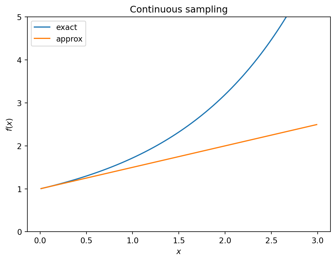
Continuous sampling
In the case of continuous sampling, where the sample taken at time \(t\) is a composite sample uniformly collected over the interval \([t - \delta t, t)\), we have: \[
\begin{align}
f(x) & = \frac{e^x - 1}{x} \\
& = 1 + \frac{x}{2} + \mathcal{O}(x^2) \\
f'(x) & \approx \frac{1}{2}
\end{align}
\] for small \(x\). Note the difference in functional form from the grab sample case.
Substituting this into the optimization equation yields: \[
{(r \delta t)}^2 \approx 2 \frac{d_s}{d_r} \frac{b \hat{c}}{\hat{K}} \left(\frac{r}{r + \beta}\right) e^{-r t_d}.
\]
Windowed composite sampling
An intermediate (and more realistic) model of sampling is windowed composite sampling. In this scheme, the sample at time \(t\) is a composite sample taken over a window of width \(w\) (e.g., 24hours) from \(t - w\) to \(t\). Notably, when the sampling interval (\(\delta t\)) increases, the length of the window does not. In this case we have:
\[
\begin{align}
f(x) & = \frac{rw}{1 - e^{-rw}} \frac{e^{-x}{(e^x - 1)}^2}{x^2} \\
& \approx \left(1 + \frac{rw}{2}\right) \frac{e^{-x}{(e^x - 1)}^2}{x^2} \\
& \approx \left(1 + \frac{rw}{2}\right) + \left(1 + \frac{rw}{2}\right) \left(\frac{x^2}{12}\right) \\
f'(x) & \approx \left(1 + \frac{rw}{2}\right) \left(\frac{x}{6}\right) \\
\end{align}
\] for small \(rw\) and \(x\). Note that as \(rw \to 0\), we recover grab sampling.
Since we’re keeping only the leading term in \(x = r \delta t\), and \(w \leq \delta t\), for consistency we should also drop the \(\frac{rw}{2}\) (or keep more terms of the expansion). Thus, we’ll treat windowed composite sampling for small windows as equivalent to grab sampling. The key reason for this is that changing the sampling interval does not change the window. Note that for \(\delta t \approx w\), i.e. \(x \approx rw\), \(f(x) \approx 1 + \frac{rw}{2}\), just as with continuous sampling, but \(f'(x)\) still behaves like grab sampling.
General properties
In general, we have: \[
r \delta t \approx {\left( a\frac{d_s}{d_r} \frac{b \hat{c}}{\hat{K}} \left(\frac{r}{r + \beta}\right) e^{-r t_d} \right)}^{1 / \gamma},
\] where \(a\) and \(\gamma\) are positive constants that depend on the sampling scheme. We can observe some general features:
Faster-growing viruses (higher \(r\)) decreases the optimal sampling interval.
Increasing the cost per sample \(d_s\)increases the optimal sampling interval.
Increasing the cost per read \(d_r\)decreases the optimal sampling interval.
Increasing the P2RA factor \(b\) or the target cumulative incidence \(c\)increases the optimal sampling interval.
Increasing the detection threshold \(\hat{K}\)decreases the optimal sampling interval.
Increasing the delay between sampling and detection \(t_d\)decreases the optimal sampling interval.
One general trend is: the more optimistic we are about our method (higher \(b\), smaller \(\hat{K}\), shorter \(t_d\)), the longer we can wait between samples.
We can also substitute our equation for \(n / \delta t\) into this equation, use \(f(\delta t) \approx 1\) and rearrange to get: \[
n d_r \approx \frac{a}{{(r \delta t)}^{\gamma - 1}} d_s.
\] The left-hand side of this equation is the cost spent on sequencing per sample. For continuous sampling, \(\gamma = 2\) and for grab sampling and windowed composite, \(\gamma = 3\). Since \(r \delta t \ll 1\), this tells us that we typically should spend more money on sequencing than sample processing.
A numerical example
Optimal \(\delta t\)
Code
import numpy as npimport matplotlib.pyplot as pltfrom typing import Optionaldef optimal_interval( per_sample_cost: float, per_read_cost: float, growth_rate: float, recovery_rate: float, read_threshold: int, p2ra_factor: float, cumulative_incidence_target: float, sampling_scheme: str, delay: float, composite_window: Optional[float] =None,) ->float: constant_term = ( (per_sample_cost / per_read_cost)* ((p2ra_factor * cumulative_incidence_target) / read_threshold)* (growth_rate / (growth_rate + recovery_rate))* np.exp(-growth_rate * delay) )if sampling_scheme =="continuous": a =2 b =2elif sampling_scheme =="grab": a =6 b =3elif sampling_scheme =="composite":ifnot composite_window:raiseValueError("For composite sampling, must provide a composite_window") a = (6* (1- np.exp(-growth_rate * composite_window))/ (growth_rate * composite_window) ) b =3else:raiseValueError("sampling_scheme must be continuous or grab")return (a * constant_term) ** (1/ b) / growth_rate
I asked the NAO in Twist for info on sequencing and sample-processing costs. Based on their answers, reasonable order-of-magnitude estimate are:
Note that 1 billion reads cost roughly 10x the cost to prepare one sample. As discussed above, our cost model is highly simplified and the specifics of when samples are collected, transported, processed, and batched for sequencing will make this calculation much more complicated in practice.
Let’s use these numbers plus our virus model from the last post to find the optimal sampling interval:
d_s =500d_r =5000*1e-9# Weekly doublingr = np.log(2) /7# Recovery in two weeksbeta =1/14# Detect when 100 cumulative readsk_hat =100# Median P2RA factor for SARS-CoV-2 in Rothmanra_i_01 =1e-7# Convert from weekly incidence to prevalence and per 1% to per 1b = ra_i_01 *100* (r + beta) *7# Goal of detecting by 1% cumulative incidencec_hat =0.01# Delay from sampling to detecting of 1 weekt_d =7.0delta_t_grab = optimal_interval(d_s, d_r, r, beta, k_hat, b, c_hat, "grab", t_d)delta_t_cont = optimal_interval(d_s, d_r, r, beta, k_hat, b, c_hat, "continuous", t_d)delta_t_24hr = optimal_interval(d_s, d_r, r, beta, k_hat, b, c_hat, "composite", t_d, 1)print(f"Optimal sampling interval with grab sampling:\t\t{delta_t_grab:.2f} days")print(f"\tr delta_t = {r*delta_t_grab:.2f}")print(f"Optimal sampling interval with continuous sampling:\t{delta_t_cont:.2f} days")print(f"\tr delta_t = {r*delta_t_cont:.2f}")print(f"Optimal sampling interval with 24-hour composite sampling:\t{delta_t_24hr:.2f} days")print(f"\tr delta_t = {r*delta_t_24hr:.2f}")
Optimal sampling interval with grab sampling:       5.98 days
    r delta_t = 0.59
Optimal sampling interval with continuous sampling: 2.66 days
    r delta_t = 0.26
Optimal sampling interval with 24-hour composite sampling:  5.89 days
    r delta_t = 0.58
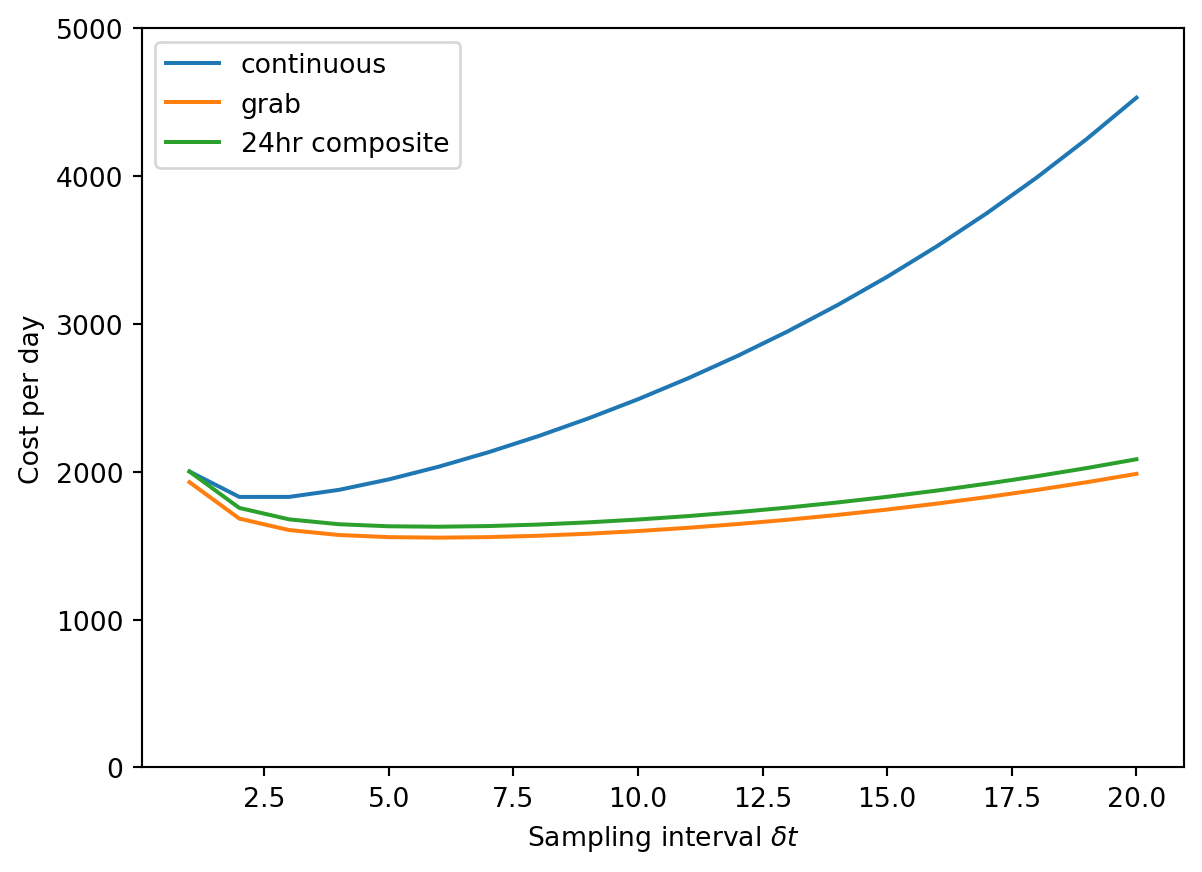
We should check that \(r \delta_t\) is small enough that our approximation for \(f(x)\) is accurate:
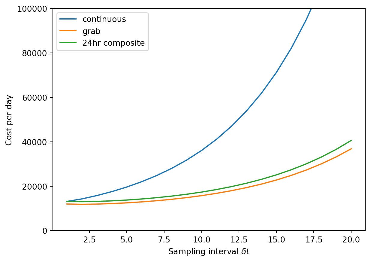
First, note that the cost of 24hr composite sampling is quite close to grab sampling, and that when the sampling interval is 1 day, it is exactly the same as continuous sampling.
It looks like the cost curve is pretty flat for the grab/24hr sampling, suggesting that we could choose a range of sampling intervals without dramatically increasing the cost. For continuous sampling, the cost increases more steeply with increasing sampling interval.
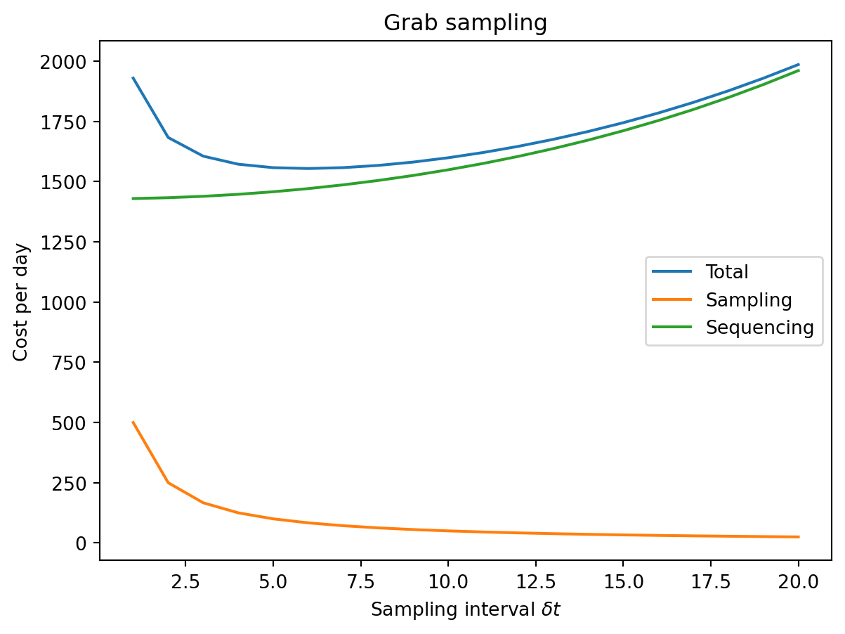
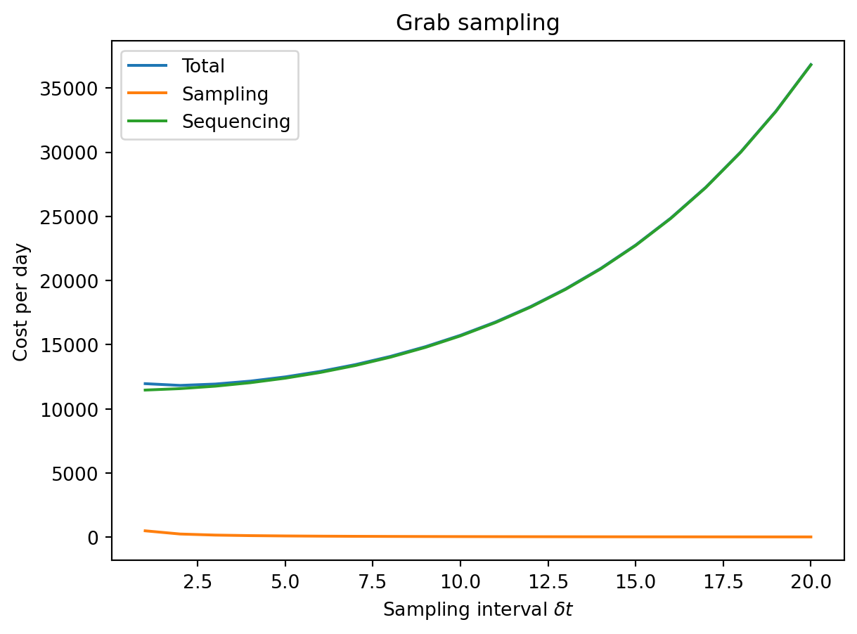
Finally, let’s break the costs down between sampling and sequencing:
Sequencing costs are always quite a bit higher than sampling costs.
Increasing the sampling interval from one day to about five generates a significant savings in sampling cost, any longer than that gives strongly diminishing returns. (This makes sense from the functional form \(d_s / \delta t\).)
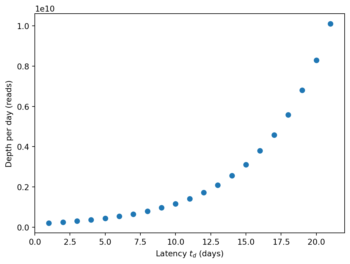
The required sequencing depth increases slowly in this range.
Sensitivity of optimal \(\delta t\) to P2RA factor
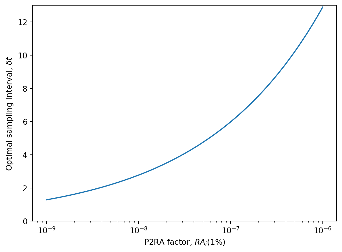
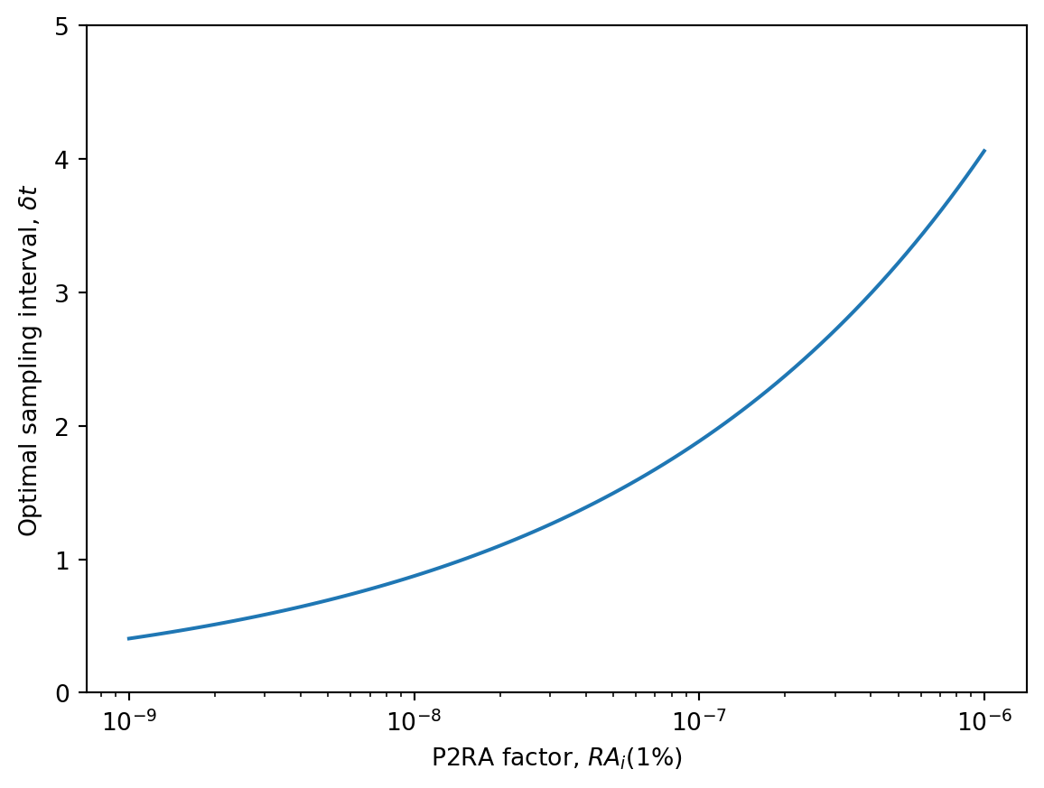
We have a lot of uncertainty in the P2RA factor, even for a specific known virus with a fixed protocol. Let’s see how the optimal sampling interval varies with it. (We’ll only do this for grab sampling.)
Code
ra_i_01 = np.logspace(-9, -6, 100)# Convert from weekly incidence to prevalence and per 1% to per 1b = ra_i_01 *100* (r + beta) *7delta_t_opt = optimal_interval(d_s, d_r, r, beta, k_hat, b, c_hat, "grab", t_d)plt.semilogx(ra_i_01, delta_t_opt)plt.xlabel("P2RA factor, $RA_i(1\%)$")plt.ylabel("Optimal sampling interval, $\delta t$")plt.ylim([0, 13])
As expected, the theory predicts that with higher P2RA factors, we can get away with wider sampling intervals. Also, for this range of P2RA factors, it never recommends daily sampling.
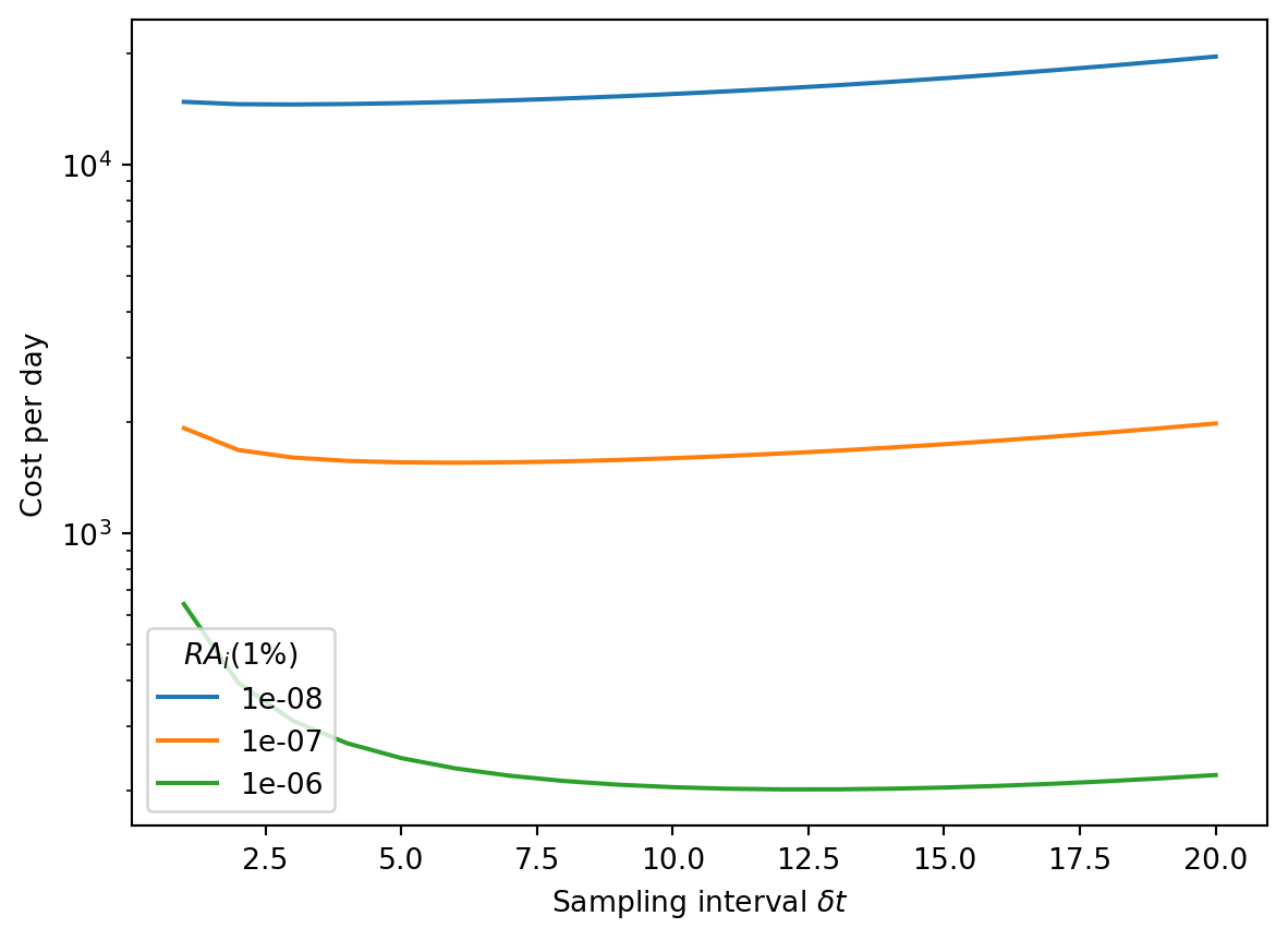
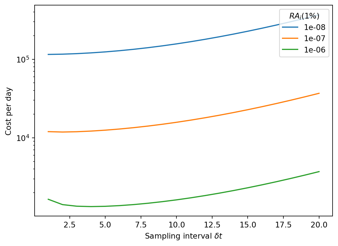
However, we can also see that the cost per day depends much more strongly on the P2RA factor than on optimizing the sampling interval:
Let’s consider a more pessimistic scenario: doubling both the growth rate and the delay to detection.
d_s =500d_r =5000*1e-9# Twice-weekly doublingr =2* np.log(2) /7# Recovery in two weeksbeta =1/14# Detect when 100 cumulative readsk_hat =100# Median P2RA factor for SARS-CoV-2 in Rothmanra_i_01 =1e-7# Convert from weekly incidence to prevalence and per 1% to per 1b = ra_i_01 *100* (r + beta) *7# Goal of detecting by 1% cumulative incidencec_hat =0.01# Delay from sampling to detecting of 2 weekst_d =14.0delta_t_grab = optimal_interval(d_s, d_r, r, beta, k_hat, b, c_hat, "grab", t_d)delta_t_cont = optimal_interval(d_s, d_r, r, beta, k_hat, b, c_hat, "continuous", t_d)delta_t_24hr = optimal_interval(d_s, d_r, r, beta, k_hat, b, c_hat, "composite", t_d, 1)print(f"Optimal sampling interval with grab sampling:\t\t{delta_t_grab:.2f} days")print(f"\tr delta_t = {r*delta_t_grab:.2f}")print(f"Optimal sampling interval with continuous sampling:\t{delta_t_cont:.2f} days")print(f"\tr delta_t = {r*delta_t_cont:.2f}")print(f"Optimal sampling interval with 24-hour composite sampling:\t{delta_t_24hr:.2f} days")print(f"\tr delta_t = {r*delta_t_24hr:.2f}")
Optimal sampling interval with grab sampling:       1.88 days
    r delta_t = 0.37
Optimal sampling interval with continuous sampling: 0.66 days
    r delta_t = 0.13
Optimal sampling interval with 24-hour composite sampling:  1.82 days
    r delta_t = 0.36
We should check that \(r \delta_t\) is small enough that our approximation for \(f(x)\) is accurate:
It looks like the cost curve is pretty flat for the grab sampling, suggesting that we could choose a range of sampling intervals without dramatically increasing the cost. For continuous sampling, the cost increases more steeply with increasing sampling interval.
Finally, let’s break the costs down between sampling and sequencing:
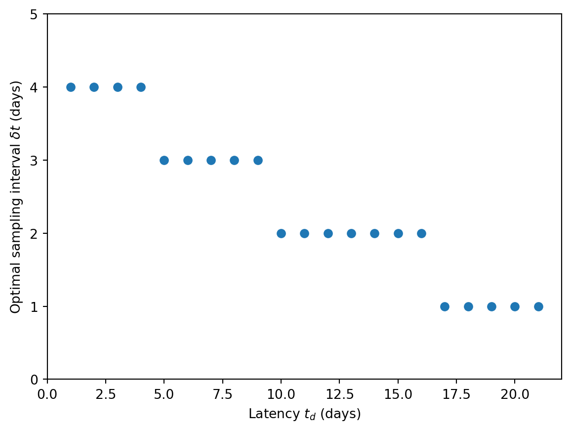
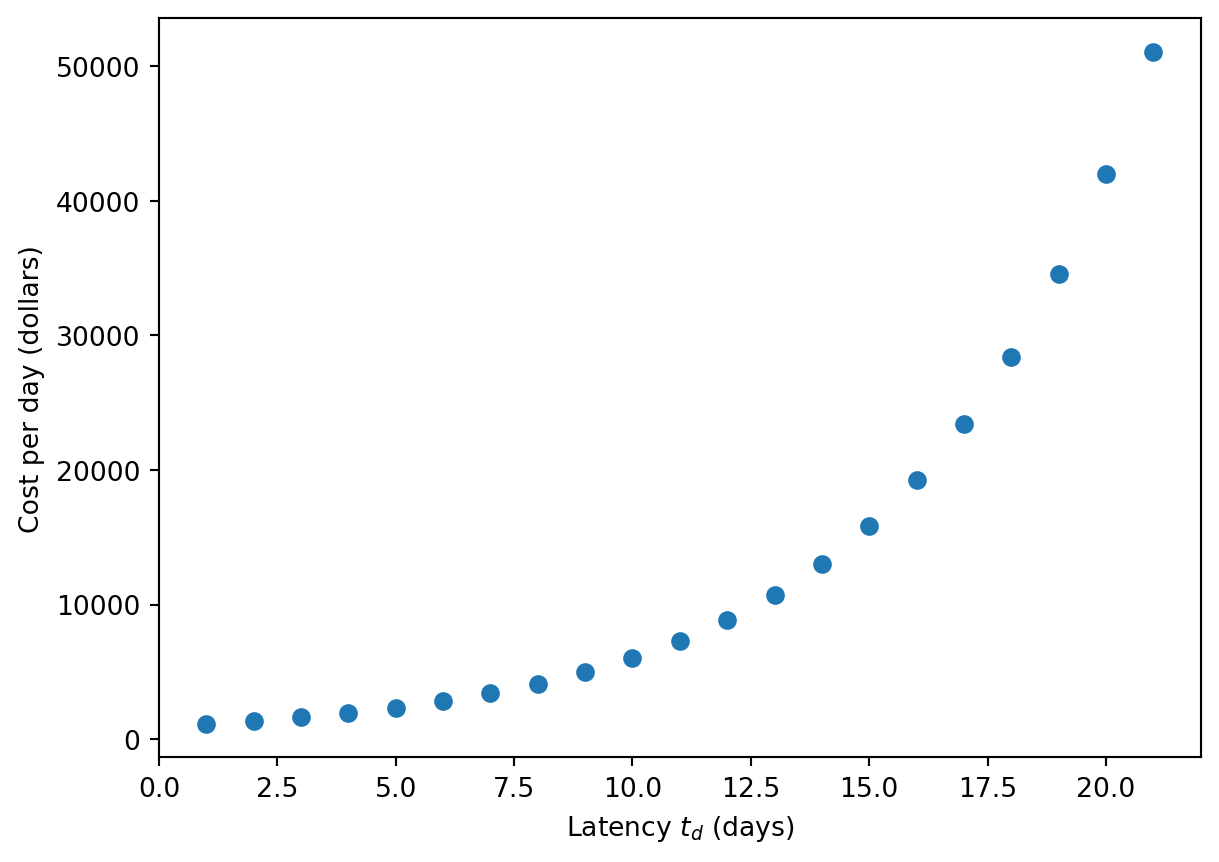
As a final application, let’s calculate what the optimal cost would be as a function of delay/latency time \(t_d\). We’ll use 24-hr composite sampling. And for some realism, we’ll round the optimal sampling interval to the nearest day.
d_s =500d_r =5000*1e-9# Bi-weekly doublingr =2* np.log(2) /7# Recovery in two weeksbeta =1/14# Detect when 100 cumulative readsk_hat =100# Median P2RA factor for SARS-CoV-2 in Rothmanra_i_01 =1e-7# Convert from weekly incidence to prevalence and per 1% to per 1b = ra_i_01 *100* (r + beta) *7# Goal of detecting by 1% cumulative incidencec_hat =0.01