Objectives
NOTE: Need sample metadata. I don’t know what the samples are.
- Test qPCR of PMMoV
- Test duplexed qPCR
- See Google Doc
Preliminary work
- Dan copied the
.eds file from the NAO qPCR data directory to the experiment directory and exported .csv files.
Data import
library(readr)
library(dplyr)
Attaching package: 'dplyr'
The following objects are masked from 'package:stats':

    filter, lag
The following objects are masked from 'package:base':

    intersect, setdiff, setequal, union
library(purrr)
library(stringr)
library(ggplot2)
library(tidyr)
library(broom)
data_dir <-
  "~/airport/[2023-09-13] PMMoV and Multiplex qPCR/"
filename_pattern <- "Results"
col_types <- list(
  Target = col_character(),
  Cq = col_double()
)
raw_data <- list.files(
  paste0(data_dir, "qpcr"),
  pattern = filename_pattern,
  full.names = TRUE,
) |>
  print() |>
  map(function(f) {
    read_csv(f,
      skip = 23,
      col_types = col_types,
    )
  }) |>
  list_rbind()
[1] "/Users/dan/airport/[2023-09-13] PMMoV and Multiplex qPCR/qpcr/Ari PMMoV_Results_20230925_115306.csv"
Warning: One or more parsing issues, call `problems()` on your data frame for details,
e.g.:
  dat <- vroom(...)
  problems(dat)
# A tibble: 63 × 21
    Well `Well Position` Omit  Sample Target Task    Reporter Quencher
   <dbl> <chr>           <lgl> <chr>  <chr>  <chr>   <chr>    <chr>
 1     1 A1              FALSE 1      PPMoV  UNKNOWN VIC      NFQ-MGB
 2     2 A2              FALSE 1      PPMoV  UNKNOWN VIC      NFQ-MGB
 3     3 A3              FALSE 1      PPMoV  UNKNOWN VIC      NFQ-MGB
 4     5 A5              FALSE 1      N2     UNKNOWN FAM      NFQ-MGB
 5     6 A6              FALSE 1      N2     UNKNOWN FAM      NFQ-MGB
 6     8 A8              FALSE NTC    N2     UNKNOWN FAM      NFQ-MGB
 7    10 A10             FALSE 1      N2     UNKNOWN FAM      NFQ-MGB
 8    10 A10             FALSE 1      PPMoV  UNKNOWN VIC      NFQ-MGB
 9    11 A11             FALSE 1      N2     UNKNOWN FAM      NFQ-MGB
10    11 A11             FALSE 1      PPMoV  UNKNOWN VIC      NFQ-MGB
# ℹ 53 more rows
# ℹ 13 more variables: `Amp Status` <chr>, `Amp Score` <dbl>,
#   `Curve Quality` <lgl>, `Result Quality Issues` <lgl>, Cq <dbl>,
#   `Cq Confidence` <dbl>, `Cq Mean` <dbl>, `Cq SD` <dbl>,
#   `Auto Threshold` <lgl>, Threshold <dbl>, `Auto Baseline` <lgl>,
#   `Baseline Start` <dbl>, `Baseline End` <dbl>
It looks like the software splits duplexed targets into two rows, but doesn’t save the information about multiplexing.
raw_data |> count(Target, Reporter, Sample, Quencher)
# A tibble: 19 × 5
   Target Reporter Sample Quencher     n
   <chr>  <chr>    <chr>  <chr>    <int>
 1 N2     FAM      1      NFQ-MGB      5
 2 N2     FAM      2      NFQ-MGB      5
 3 N2     FAM      NTC    NFQ-MGB      2
 4 N2     FAM      SC1    NFQ-MGB      3
 5 N2     FAM      SC2    NFQ-MGB      3
 6 N2     FAM      SC3    NFQ-MGB      3
 7 N2     FAM      SC4    NFQ-MGB      3
 8 N2     FAM      SC5    NFQ-MGB      3
 9 N2     FAM      SC6    NFQ-MGB      3
10 N2     FAM      <NA>   NFQ-MGB      2
11 PPMoV  VIC      1      NFQ-MGB      6
12 PPMoV  VIC      2      NFQ-MGB      6
13 PPMoV  VIC      NTC    NFQ-MGB      4
14 PPMoV  VIC      SC1    NFQ-MGB      1
15 PPMoV  VIC      SC2    NFQ-MGB      3
16 PPMoV  VIC      SC3    NFQ-MGB      3
17 PPMoV  VIC      SC4    NFQ-MGB      3
18 PPMoV  VIC      SC5    NFQ-MGB      3
19 PPMoV  VIC      <NA>   NFQ-MGB      2
raw_data |>
  count(`Well Position`) |>
  print(n = Inf)
# A tibble: 54 × 2
   `Well Position`     n
   <chr>           <int>
 1 A1                  1
 2 A10                 2
 3 A11                 2
 4 A12                 2
 5 A2                  1
 6 A3                  1
 7 A5                  1
 8 A6                  1
 9 A8                  1
10 B1                  1
11 B10                 2
12 B11                 2
13 B12                 2
14 B2                  1
15 B3                  1
16 B5                  1
17 B6                  1
18 C1                  1
19 C10                 2
20 C11                 2
21 C12                 2
22 C2                  1
23 C3                  1
24 C5                  1
25 C6                  1
26 C7                  1
27 D3                  1
28 D5                  1
29 D6                  1
30 D7                  1
31 E1                  1
32 E2                  1
33 E3                  1
34 E5                  1
35 E6                  1
36 E7                  1
37 F1                  1
38 F2                  1
39 F3                  1
40 F5                  1
41 F6                  1
42 F7                  1
43 G1                  1
44 G2                  1
45 G3                  1
46 G5                  1
47 G6                  1
48 G7                  1
49 H1                  1
50 H2                  1
51 H3                  1
52 H5                  1
53 H6                  1
54 H7                  1
We can count the multiplexing and save it as a column:
with_counts <- raw_data |>
  left_join(count(raw_data, Well, name = "n_multiplex"), by = join_by(Well))
It looks like the multiplexed wells didn’t amplifiy well. No N2 wells amplified. It also looks like there was poor amp in general.
with_counts |>
  count(Target, Reporter, Sample, n_multiplex, `Amp Status`) |>
  print(n = Inf)
# A tibble: 32 × 6
   Target Reporter Sample n_multiplex `Amp Status`     n
   <chr>  <chr>    <chr>        <int> <chr>        <int>
 1 N2     FAM      1                1 AMP              1
 2 N2     FAM      1                1 NO_AMP           1
 3 N2     FAM      1                2 NO_AMP           3
 4 N2     FAM      2                1 NO_AMP           2
 5 N2     FAM      2                2 NO_AMP           3
 6 N2     FAM      NTC              1 NO_AMP           1
 7 N2     FAM      NTC              2 NO_AMP           1
 8 N2     FAM      SC1              1 AMP              1
 9 N2     FAM      SC1              1 NO_AMP           2
10 N2     FAM      SC2              1 AMP              2
11 N2     FAM      SC2              1 NO_AMP           1
12 N2     FAM      SC3              1 AMP              2
13 N2     FAM      SC3              1 NO_AMP           1
14 N2     FAM      SC4              1 AMP              2
15 N2     FAM      SC4              1 NO_AMP           1
16 N2     FAM      SC5              1 AMP              2
17 N2     FAM      SC5              1 NO_AMP           1
18 N2     FAM      SC6              1 AMP              1
19 N2     FAM      SC6              1 NO_AMP           2
20 N2     FAM      <NA>             2 NO_AMP           2
21 PPMoV  VIC      1                1 AMP              3
22 PPMoV  VIC      1                2 AMP              3
23 PPMoV  VIC      2                1 AMP              3
24 PPMoV  VIC      2                2 AMP              3
25 PPMoV  VIC      NTC              1 NO_AMP           3
26 PPMoV  VIC      NTC              2 NO_AMP           1
27 PPMoV  VIC      SC1              1 AMP              1
28 PPMoV  VIC      SC2              1 AMP              3
29 PPMoV  VIC      SC3              1 AMP              3
30 PPMoV  VIC      SC4              1 AMP              3
31 PPMoV  VIC      SC5              1 AMP              3
32 PPMoV  VIC      <NA>             2 NO_AMP           2
with_counts |>
  count(Target, n_multiplex, `Amp Status`) |>
  print(n = Inf)
# A tibble: 7 × 4
  Target n_multiplex `Amp Status`     n
  <chr>        <int> <chr>        <int>
1 N2               1 AMP             11
2 N2               1 NO_AMP          12
3 N2               2 NO_AMP           9
4 PPMoV            1 AMP             19
5 PPMoV            1 NO_AMP           3
6 PPMoV            2 AMP              6
7 PPMoV            2 NO_AMP           3
Check that the thresholds are the same for every well with the same target
with_counts |>
  count(Target, Threshold) |>
  print(n = Inf)
# A tibble: 2 × 3
  Target Threshold     n
  <chr>      <dbl> <int>
1 N2          5.82    32
2 PPMoV       1.53    31
Amplification curves
amp_data <- list.files(
  paste0(data_dir, "qpcr"),
  pattern = "Amplification Data",
  full.names = TRUE,
) |>
  map(function(f) {
    read_csv(f,
      skip = 23,
      col_types = col_types,
    )
  }) |>
  list_rbind() |>
  left_join(with_counts,
    by = join_by(Well, `Well Position`, Sample, Target)
  ) |>
  print()
Warning: The following named parsers don't match the column names: Cq
# A tibble: 2,520 × 26
    Well `Well Position` `Cycle Number` Target    Rn     dRn Sample Omit.x
   <dbl> <chr>                    <dbl> <chr>  <dbl>   <dbl> <chr>  <lgl>
 1     1 A1                           1 PPMoV   13.5 -1.41   1      FALSE
 2     1 A1                           2 PPMoV   13.8 -1.23   1      FALSE
 3     1 A1                           3 PPMoV   14.4 -0.752  1      FALSE
 4     1 A1                           4 PPMoV   14.8 -0.474  1      FALSE
 5     1 A1                           5 PPMoV   15.2 -0.290  1      FALSE
 6     1 A1                           6 PPMoV   15.5 -0.0864 1      FALSE
 7     1 A1                           7 PPMoV   15.8  0.0333 1      FALSE
 8     1 A1                           8 PPMoV   16.0  0.138  1      FALSE
 9     1 A1                           9 PPMoV   16.3  0.272  1      FALSE
10     1 A1                          10 PPMoV   16.5  0.302  1      FALSE
# ℹ 2,510 more rows
# ℹ 18 more variables: Omit.y <lgl>, Task <chr>, Reporter <chr>,
#   Quencher <chr>, `Amp Status` <chr>, `Amp Score` <dbl>,
#   `Curve Quality` <lgl>, `Result Quality Issues` <lgl>, Cq <dbl>,
#   `Cq Confidence` <dbl>, `Cq Mean` <dbl>, `Cq SD` <dbl>,
#   `Auto Threshold` <lgl>, Threshold <dbl>, `Auto Baseline` <lgl>,
#   `Baseline Start` <dbl>, `Baseline End` <dbl>, n_multiplex <int>
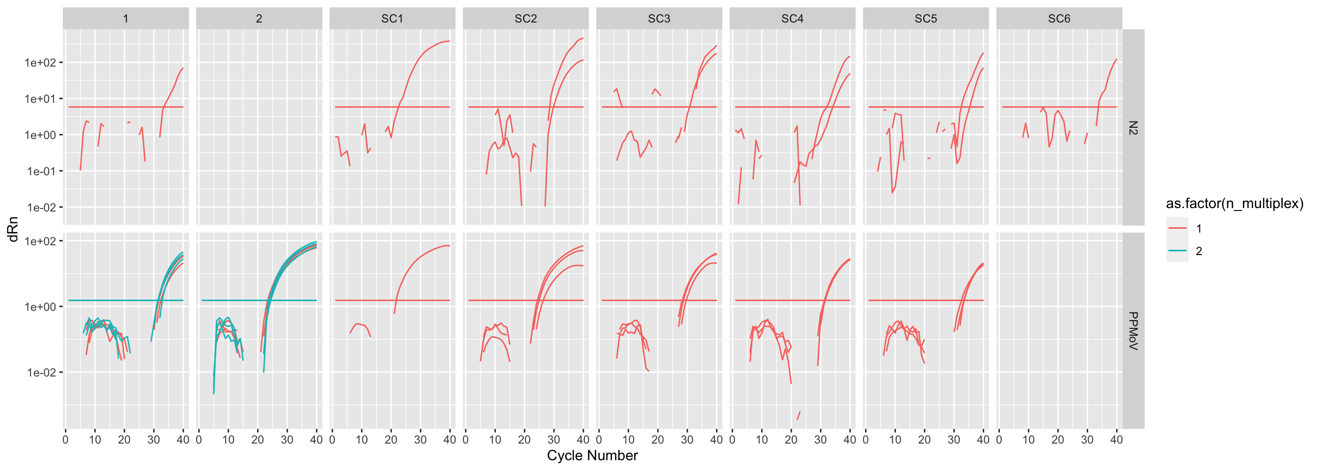
Amplification curves by sample
The one that amplified:
amp_data |>
  filter(`Amp Status` == "AMP") |>
  ggplot(mapping = aes(
    x = `Cycle Number`,
    y = dRn,
    group = Well,
    color = as.factor(n_multiplex),
  )) +
  geom_line() +
  geom_line(mapping = aes(
    x = `Cycle Number`,
    y = Threshold,
  )) +
  scale_y_log10() +
  facet_grid(
    rows = vars(Target), cols = vars(Sample), scales = "free_y"
  )
Warning in self$trans$transform(x): NaNs produced
Warning: Transformation introduced infinite values in continuous y-axis
Warning: Removed 169 rows containing missing values (`geom_line()`).
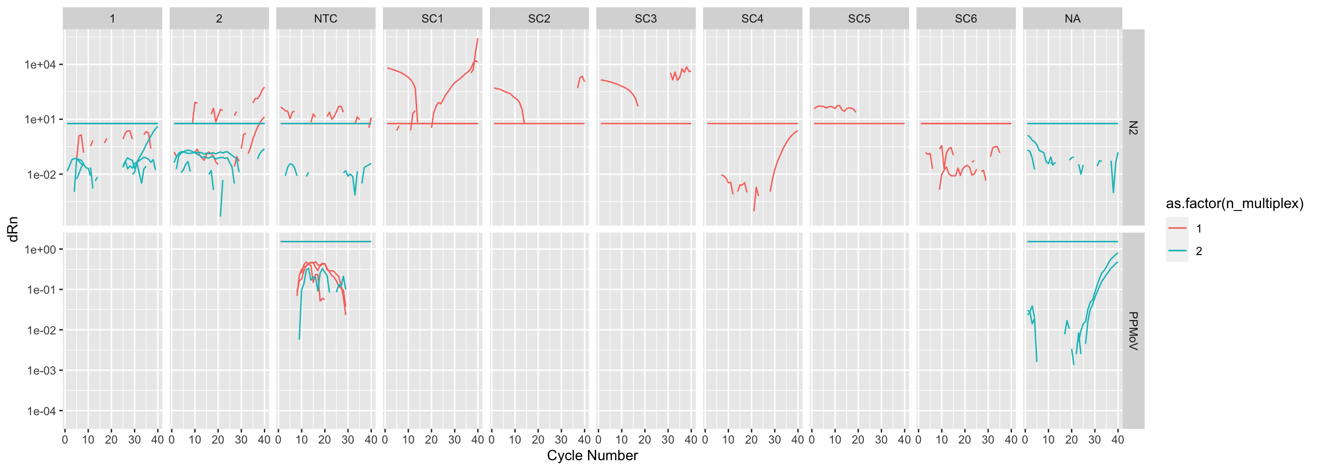
The ones that didn’t:
amp_data |>
  filter(`Amp Status` == "NO_AMP") |>
  ggplot(mapping = aes(
    x = `Cycle Number`,
    y = dRn,
    group = Well,
    color = as.factor(n_multiplex),
  )) +
  geom_line() +
  geom_line(mapping = aes(
    x = `Cycle Number`,
    y = Threshold,
  )) +
  scale_y_log10() +
  facet_grid(
    rows = vars(Target), cols = vars(Sample), scales = "free_y"
  )
Warning in self$trans$transform(x): NaNs produced
Warning: Transformation introduced infinite values in continuous y-axis
Warning: Removed 187 rows containing missing values (`geom_line()`).
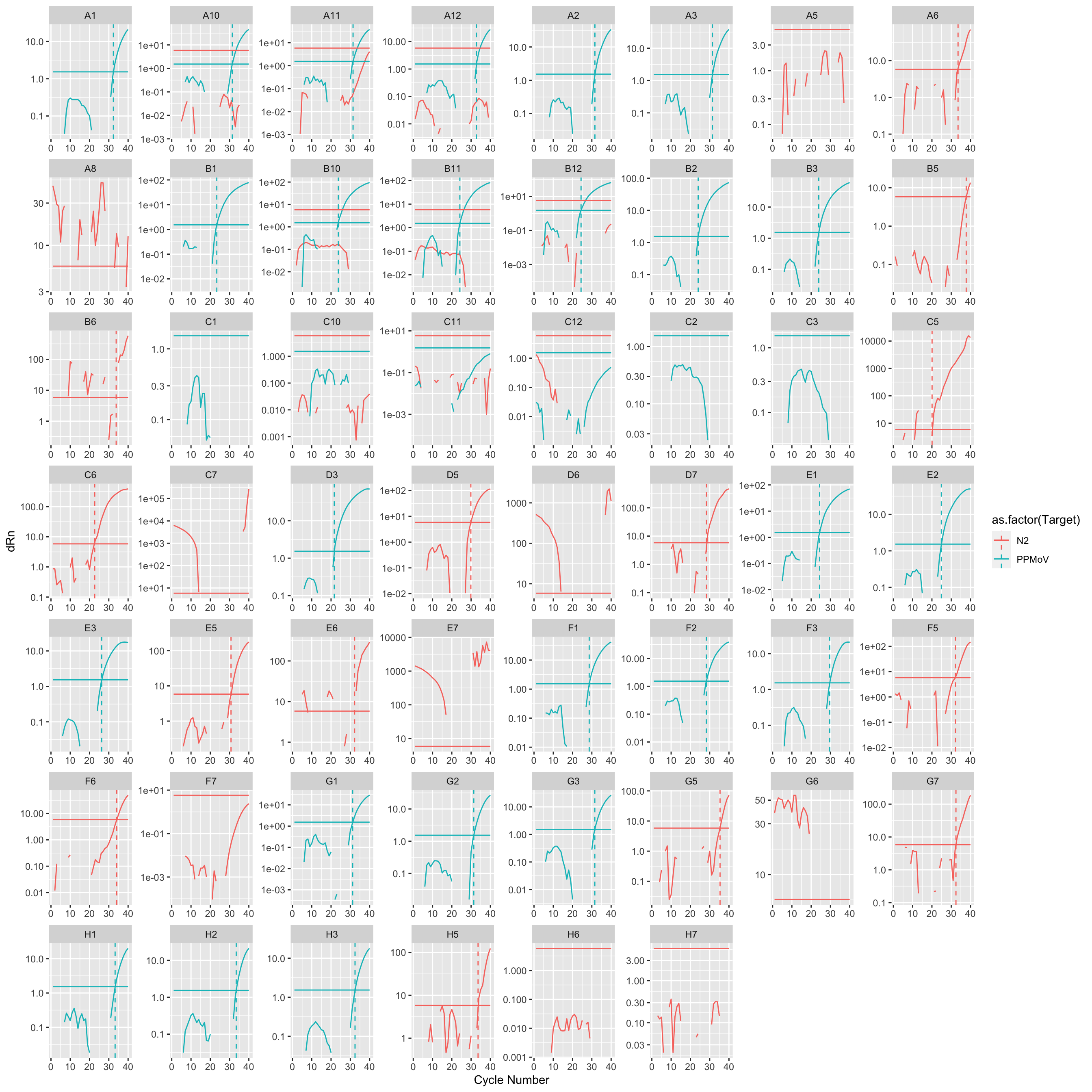
Amplification curves by well
amp_data |>
  ggplot(mapping = aes(
    x = `Cycle Number`,
    y = dRn,
    color = as.factor(Target),
  )) +
  geom_line() +
  geom_line(mapping = aes(
    x = `Cycle Number`,
    y = Threshold
  )) +
  geom_vline(aes(xintercept = `Cq`, color = as.factor(Target)),
    linetype = "dashed"
  ) +
  scale_y_log10() +
  facet_wrap(~`Well Position`, scales = "free")
Warning in self$trans$transform(x): NaNs produced
Warning: Transformation introduced infinite values in continuous y-axis
Warning: Removed 15 rows containing missing values (`geom_line()`).
Warning: Removed 960 rows containing missing values (`geom_vline()`).